The Excel PERCENTOF function simplifies calculating percentages in Excel.
Percentage calculations are some of the most commonly used formulas in Excel, so having a function provided for this purpose makes complete sense. Some users find percentage formulas tricky, but PERCENTOF removes many of these obstacles.
The PERCENTOF function is also a function in the amazing GROUPBY and PIVOTBY functions making it even easier to build single formula reports in Excel with percentage calculations.
In this article, we will start with some basic, though very useful examples, and finish with more advanced examples with PERCENTOF used in the GROUPBY and PIVOTBY functions.
Download the practise file to follow along.
PERCENTOF Function in Excel
The PERCENTOF function returns what percentage one number is of another. It only requires the two numbers to be used in the calculation.
The syntax for the PERCENTOF function is as follows.
=PERCENTOF(data_subset, data_all)
Data subset: This value is the numerator in the percentage calculation. It is often also referred to as the part (when dividing a part by its whole), the subset value, or the new value (when performing percentage change calculations.)
Data all: This value is the denominator in the percentage calculation. It is often referred to as the whole (when dividing a part by its whole), the total value, or the old value (when performing percentage change formulas.)
Let’s get to the formula examples.
Watch the Video
Calculate Percent of Total Value
Let’s start with a classic Excel formula, calculating the percentage of total (we will do this with a single GROUPBY formula later in this tutorial.)
The following PERCENTOF formula is used to return the percentage contribution of each region to the total in cell C2.
=PERCENTOF([@[Units Sold]],C$2)
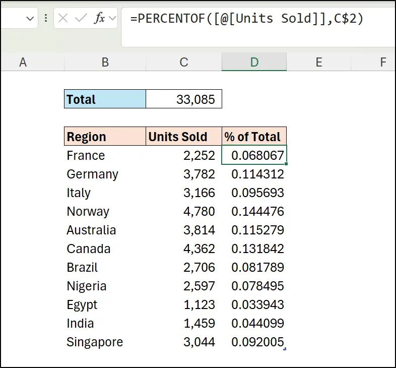
The dollar sign in the C$2 address makes it a fixed cell referenced by each units sold total. The @ symbol in the Units Sold column reference indicates that it is referencing only the units sold value on that row, and not all units sold values.
Apply the Percentage Format
The formula does not return the results in percentage format, so that is a task for us now.
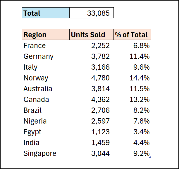
Select the values to format. This can be done quickly by clicking a cell in the percent of total column and pressing Ctrl + Space. Then click the Percent Style button on the Home tab, or press Ctrl + Shift + %.
You can add decimal values if desired by clicking the Increase Decimal button in the Number group of the Home tab.
It looks a lot better with the percentage format applied.
Excel Percentage Formula for % Change
Percentage change formulas are another really common use case for this function. And this formula can be tricky for some users, as you need to calculate the value difference first before performing the percentage calculation (the division.)
With PERCENTOF, users are shielded from those more complex calculations.
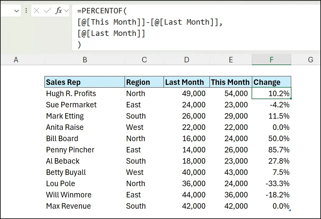
In this PERCENTOF formula, we have returned the percentage change between the This Month and Last Month columns.
=PERCENTOF(
[@[This Month]]-[@[Last Month]],
[@[Last Month]]
)
Without PERCENTOF, the difference calculation would have required brackets to ensure that it is calculated first. PERCENTOF protects users from knowing elements such as this.
=([@[This Month]]-[@[Last Month]])/[@[Last Month]]
PERCENTOF Function with GROUPBY
Calculating percentages is easy with the GROUPBY function as PERCENTOF is one of the 17 functions in its function list.
GROUPBY is an Excel function to produce summary reports from a single formula. At a minimum, it requires a columns of labels, a values column and then an aggregation function to perform for each label.
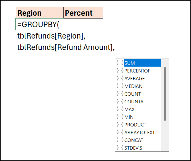
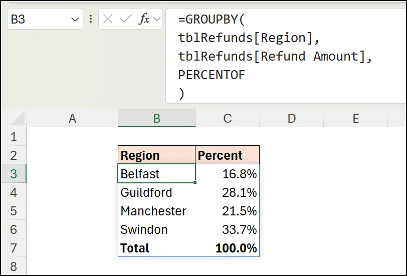
The following Excel percentage formula is a complete report produced by a single Excel formula, thanks to GROUPBY. It calculates the percentage of total for each region.
=GROUPBY(
tblRefunds[Region],
tblRefunds[Refund Amount],
PERCENTOF
)
The percentage format was applied to the cells manually and are not returned as part of the function.
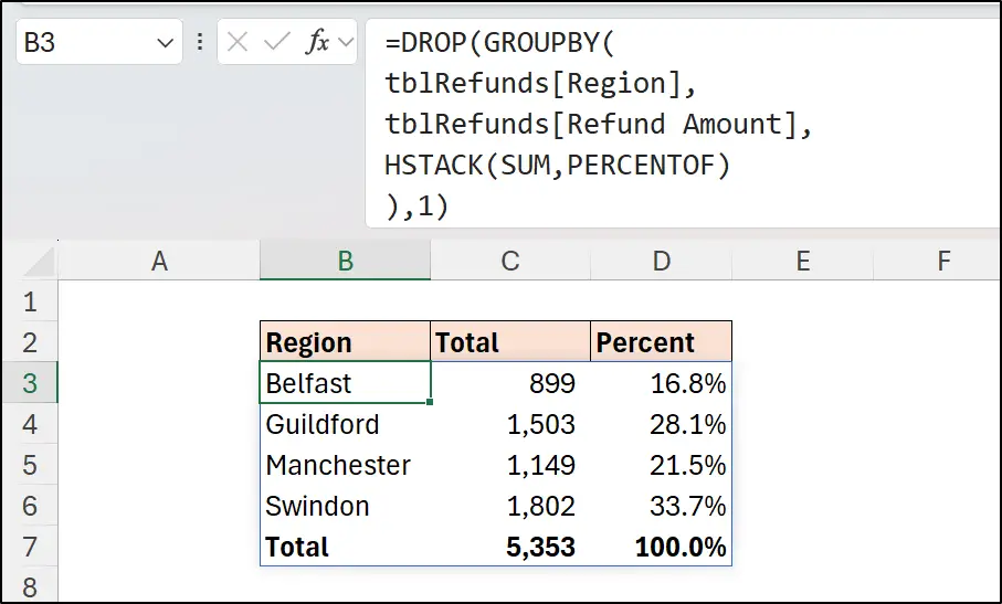
We can take this example to another level and display the sum and the percentage formula using the HSTACK function.
=DROP(GROUPBY(
tblRefunds[Region],
tblRefunds[Refund Amount],
HSTACK(SUM,PERCENTOF)
),1)
The DROP function is also included in the formula. This is used to remove the first row from the formula results, otherwise, when using HSTACK within GROUPBY, headers for each calculation column are automatically generated.
I do not want to stray too much from the topic of using the PERCENTOF function to calculate percentages in Excel, but felt that you would be interested in how to show the percentage values in addition to the sum.
PERCENTOF with the PIVOTBY Function
PERCENTOF is also included in the function list of the PIVOTBY Excel formula.
And this function takes it further than GROUPBY as PIVOTBY has a relative to argument, which enables you to calculate the percentage to a specific level of your pivot-style report, such as the grand total, row subtotals, or column subtotals.
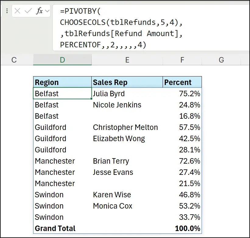
In this percentage formula, the PIVOTBY function is used with two columns (region and sales rep) for its row fields and the subtotal for rows is shown. In its default state, you can see that the percentage calculations are relative to the grand total.
=PIVOTBY(
CHOOSECOLS(tblRefunds,5,4),
,tblRefunds[Refund Amount],
PERCENTOF,,2)

If you’re new to the PIVOTBY function, it is worthwhile to read more on this brilliant Excel function.
However, for some context for now, the CHOOSECOLS function is used to extract the fifth and fourth columns from the tblRefunds table to the row fields argument. The number 2 at the end of the function is used to specify the use of subtotals below the group.
Percent Relative to Parent Row Total
To switch the function to calculate the percentage to the subtotals instead of the grand total, we can use the relative to argument of PIVOTBY.
In the following formula, the number 4 at the end of the PIVOTBY function specifies the parent row total option. So, at both the sales rep level and at the region subtotal level, PERCENTOF is used to calculate the percentage to its parent row total.
=PIVOTBY(
CHOOSECOLS(tblRefunds,5,4),
,tblRefunds[Refund Amount],
PERCENTOF,,2,,,,,4)
Summary
Calculating percentages in Microsoft Excel is easier with the PERCENTOF function.
This is a very useful function for the billions of Excel users worldwide. And for the advanced Excel users, its role within the PIVOTBY function, in particular, is a great one.
It has never been easier to calculate percentages in Excel.


