The GROUPBY function in Excel was released at the same time as the PIVOTBY function to make single formula reports simple.
In this tutorial, you will learn all the details of the GROUPBY function along with multiple examples.
Download the practise file to follow along.
GROUPBY Function in Excel
With GROUPBY, you can group rows (such as region, product category, or manager) and return aggregate values (such as the sum, average, count or percentage of) for each of those rows.
In a nutshell, simple pivot table style reports but from only one formula.
The syntax of the GROUPBY function is as follows.
=GROUPBY(row_fields, values, function, [field_headers], [total_depth], [sort_order], [filter_array], [field_relationship])
- Row fields: The columns you want to use for the row values.
- Values: The columns that the aggregation function will be applied to.
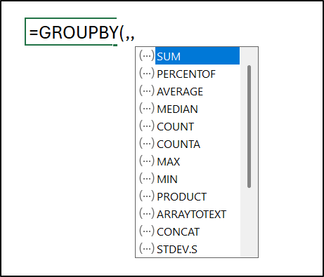
- Function: The function to apply to the values. GROUPBY provides 17 aggregation functions including SUM, COUNT, ARRAYTOTEXT and even LAMBDA functions.
- [Field headers]: Do you want to return the field headers from the source data?
- [Total depth]: Do you want to show the grand total and subtotals? And would you like them shown at the top or bottom of the group? The subtotals will only be an option when using multiple columns for the row fields argument.
- [Sort order]: How would you like the results to be ordered? Enter an index number that corresponds to the columns in row fields followed by values. Enter a positive number for ascending order and a negative number for descending order. For example, entering -2 states to sort the results in descending order by the second column.
- [Filter array]: A filter expression to determine the rows to return e.g., tblSales[Country]=”Jamaica”.
- [Field relationship]: When using multiple columns for row fields, this specifies the relationship between the columns. The options are 0 for Hierarchy (default) or 1 for Table. With the hierarchy, the sorting of later columns respects the hierarchy of earlier columns. With Table, the sorting of each column is made independently.
Data Set for GROUPBY Function Examples
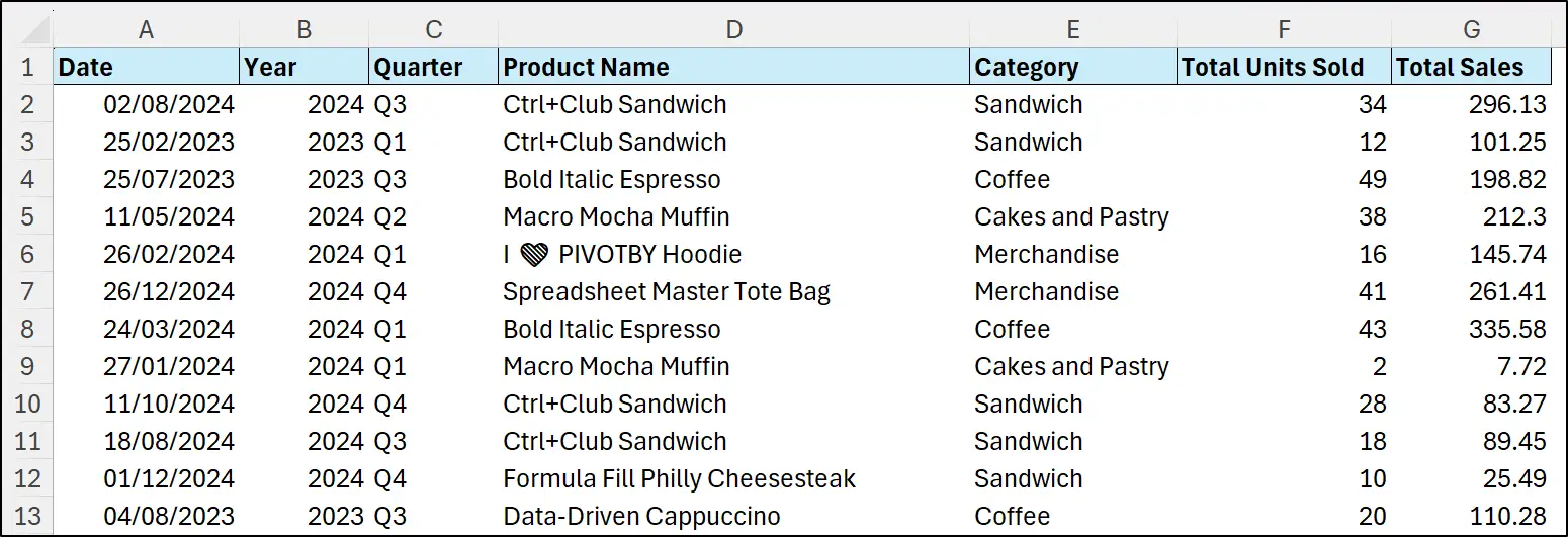
For the GROUPBY function examples in this tutorial, we will be using the following table, named tblSales, as our source data. It contains 300 rows of sales of Excel-themed coffee shop products.
Simple GROUPBY Formula
Let’s begin with a simple example of GROUPBY being used to summarise data.
The following formula returns the sum of total sales for each product name. The minimum information has been given to GROUPBY for this – ‘Product Name’ column for the row fields, ‘Total Sales’ column for the values, and to use SUM as the function.
=GROUPBY(tblSales[Product Name],tblSales[Total Sales],SUM)
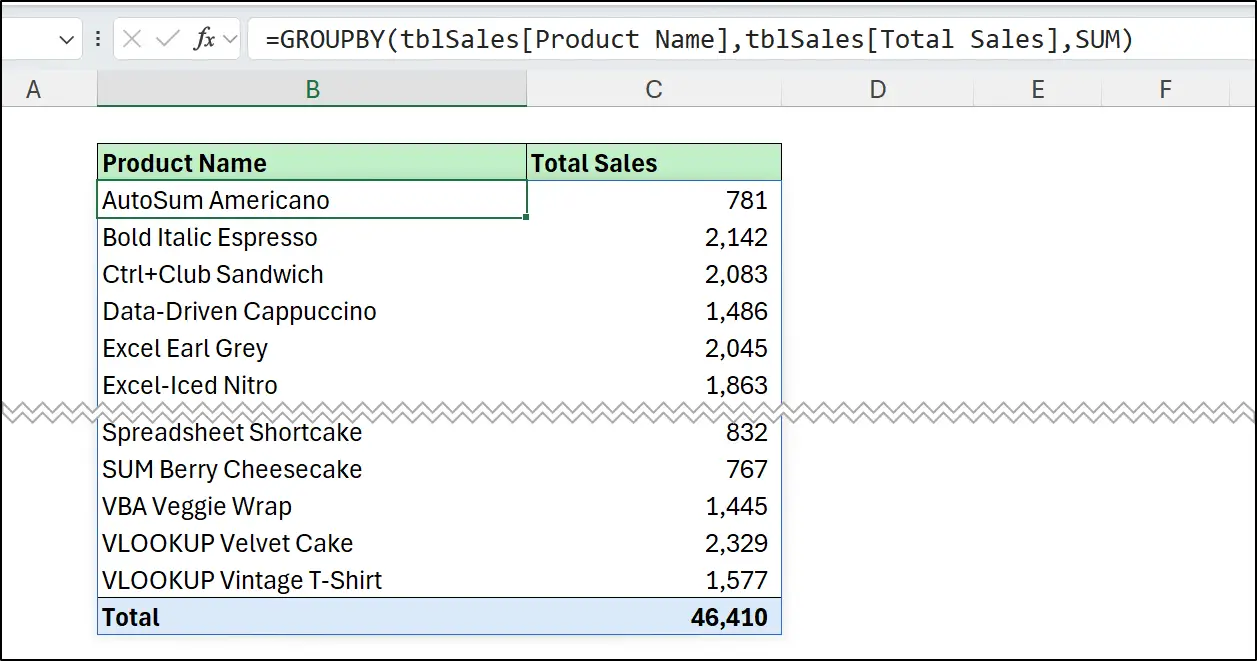
Formatting cannot be returned by the formula, so the initial results will not look as appealing as those of a pivot table. However, Conditional Formatting rules can be established to automatically apply the appropriate formatting to elements of the GROUPBY results e.g., the total row as shown in the image above.
Sorting the Grouped Data
The results of the GROUPBY function are displayed in ascending order of the first row fields column by default. Let’s look at how we can change this.
If we want to sort the results of the previous formula in largest to smallest order of the ‘Total Sales’ column, a negative 2 should be entered for the sort order.
=GROUPBY(tblSales[Product Name],tblSales[Total Sales],SUM,,,-2)
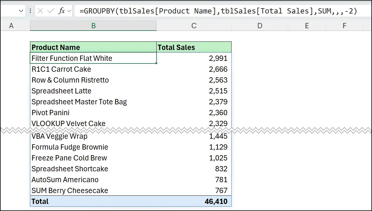
Remember, to sort the results of an Excel GROUPBY function, you enter the column number to sort by (in the order of row fields followed by values fields). A positive value specifies ascending order and a negative value specifies descending order.
In this formula, multiple row fields have been used – ‘Product Name’ and ‘Category’. The 2 in the sort order argument states to sort the results by the ‘Category’ column in A to Z order. The 1 on the end states to use the Table field relationship instead of the Hierarchy.
=GROUPBY(tblSales[[Product Name]:[Category]],tblSales[Total Sales],SUM,,,2,,1)
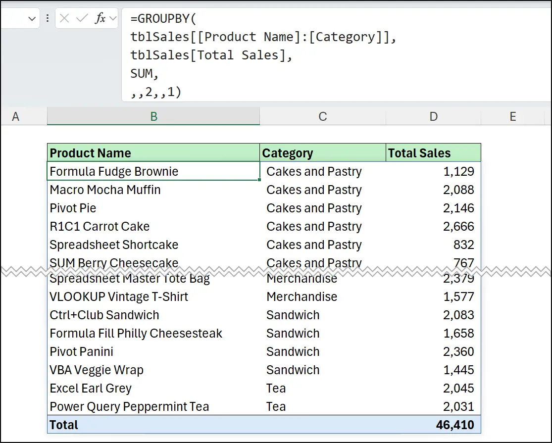
Specifying the Table field relationship in this example was essential for its operation. Without it, a Hierarchy is used and the first row field – ‘Product Name’ would have taken priority and prevented the ‘Category’ column from driving the order.
Choosing Specific Columns for use as Row Fields
The previous example showed multiple columns being used in the row fields argument of GROUPBY. This is great, but natively, GROUPBY only allows the selection of adjacent columns.
To choose the columns you want and in the order you want to use them, you can use the CHOOSECOLS function in Excel.
In the following formula, CHOOSECOLS is used to specify the use of the ‘Category’ and ‘Product Name’ columns for GROUPBY. This time, by using the CHOOSECOLS function, we were able to reverse the order that they are shown in the Excel GROUPBY formula results.
=GROUPBY(
CHOOSECOLS(tblSales,5,4),
tblSales[Total Sales],
SUM,,,-3)
In the CHOOSECOLS function, the tblSales table was given and column 5 followed by column 4 was requested. In the GROUPBY function, a negative 3 is used to sort the results by the ‘Total Sales’ column in largest to smallest order.
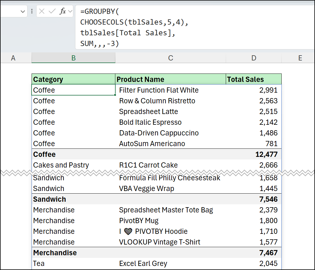
On changing the order of the columns, the GROUPBY function automatically returned subtotals for the categories. This is awesome, but we should look at how we can exclude grand total rows and change how subtotals are displayed.
Showing Subtotals in Formula Results
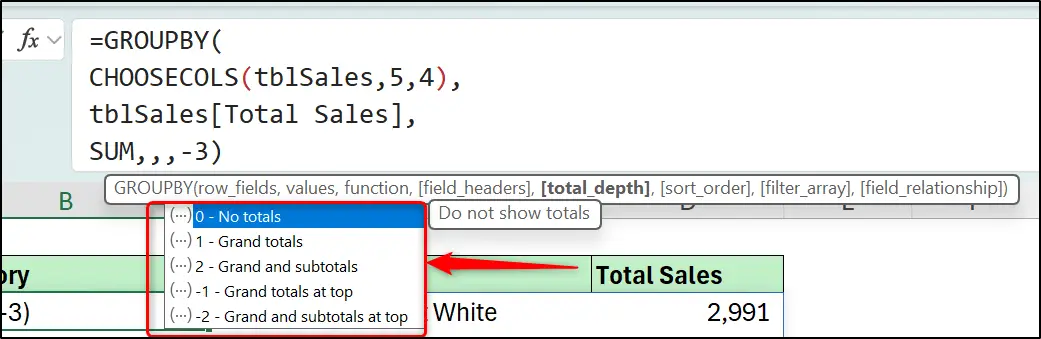
The display of subtotal and grand total rows is controlled by the total depth argument of the GROUPBY function.
There are five options for GROUPBY totals and they cover all instances from no totals, if subtotals are displayed or not, and if the grand total and subtotals are shown at the top of the group or below the group.
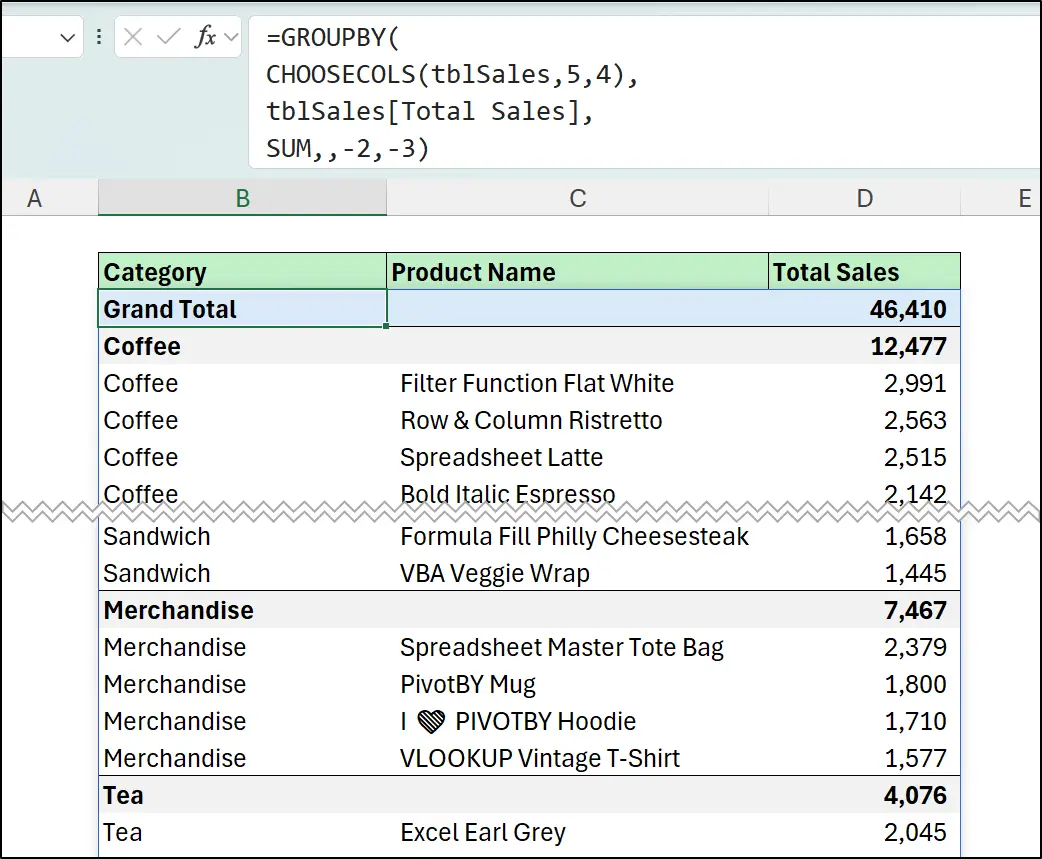
In the following formula, the grand totals and subtotals are shown at the top of the grouped rows. This is specified by the -2 option in the Excel formula.
=GROUPBY(
CHOOSECOLS(tblSales,5,4),
tblSales[Total Sales],
SUM,,-2,-3)
Filtering GROUPBY Results
The filter array argument of the Excel GROUPBY function enables you to filter data based on given conditions.
This argument can be used in the same way as the include argument of the FILTER function. You can set filters based on cell values, utilise AND and OR logic, and much more.
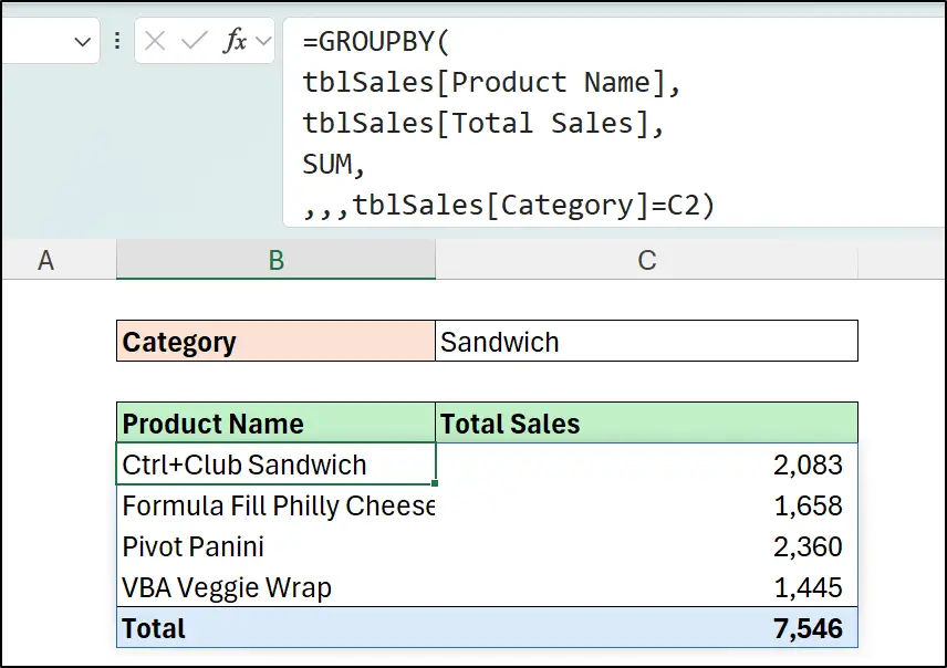
For this formula example, a condition is given to filter the data based on the category being equal to the value in cell C2. This cell contains a drop-down list making it easy for the user to change the category.
=GROUPBY(
tblSales[Product Name],
tblSales[Total Sales],
SUM,
,,,tblSales[Category]=C2)
Using GROUPBY with Slicers
For excel users of pivot tables, a common question is “can you use Slicers with the Excel GROUPBY function?”, and the answer, of course, is absolutely.
To use the GROUPBY function with Slicers, the AGGREGATE function is used to connect the Slicer and the formula together. The AGGREGATE function is the glue between the GROUPBY function and the table that the Slicers is operating on.
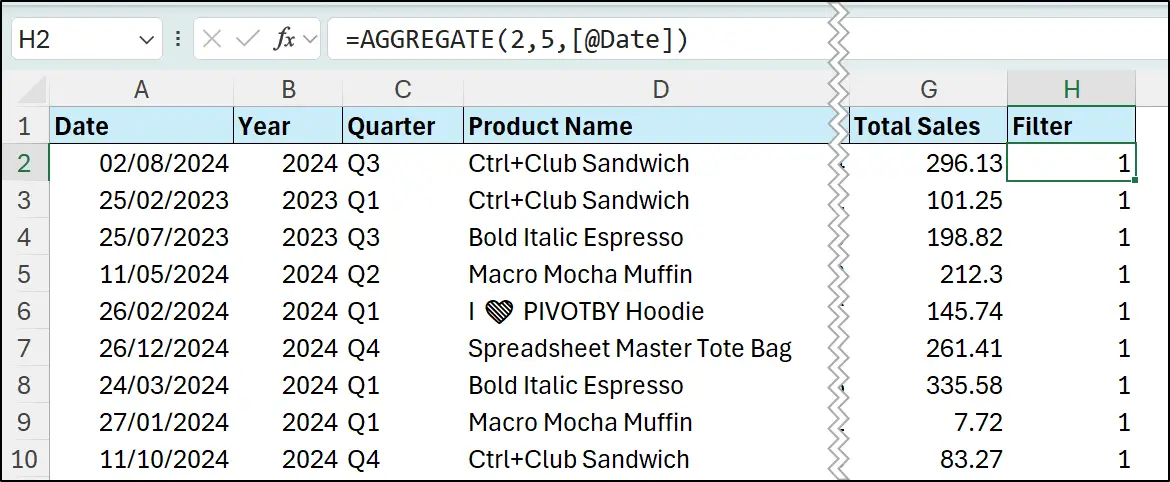
The following formula has been added as a new column, named Filter, to the source data. It uses the COUNT function (option 2) on each date value in the Date column while ignoring hidden rows (option 5).
=AGGREGATE(2,5,[@Date])
So essentially, it counts the row only if it is visible (not filtered by the Slicer). In the image, you can see the number 1 down the Filter column, because these are visible rows. If the row was filtered out, it would contain a 0, though you would not see this.
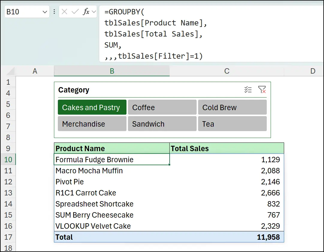
With the AGGREGATE function playing the role of flagging the visible rows, we can now write a GROUPBY function and filter for the rows that have a 1 in the Filter column. Oh, and of course insert a Slicer to filter the source table.
=GROUPBY(
tblSales[Product Name],
tblSales[Total Sales],
SUM,
,,,tblSales[Filter]=1)
Multiple Function Columns with the GROUPBY Function
In all GROUPBY function examples so far, SUM has been used to aggregate values of GROUPBY. However, you may recall that GROUPBY can handle 17 different aggregation functions. And we could have picked any of these as alternative examples to SUM.
To make things more interesting for this final example, we will use the HSTACK function to enable us to use the GROUPBY function with multiple functions.
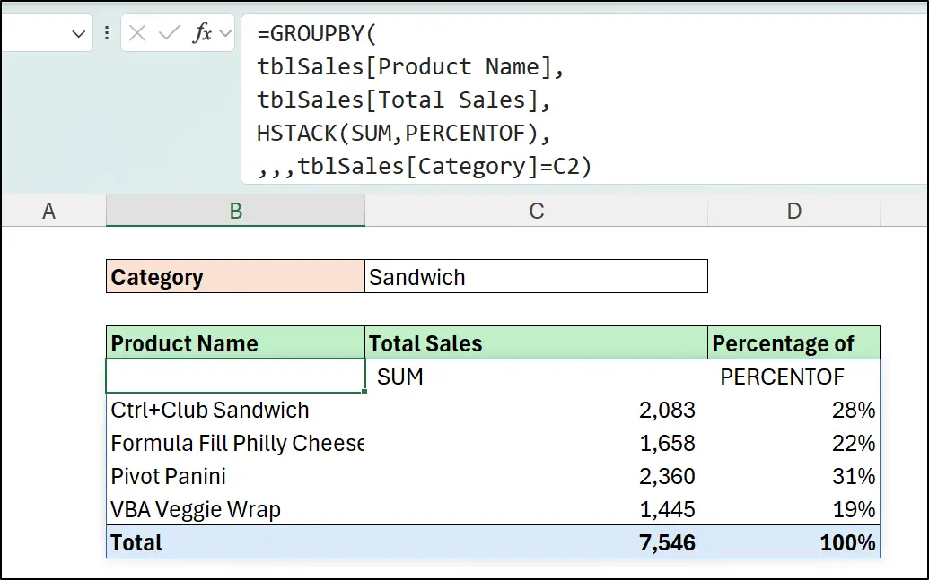
In the following formula, the SUM and PERCENTOF function have both been used for the function argument, thanks to the help of HSTACK.
=GROUPBY(
tblSales[Product Name],
tblSales[Total Sales],
HSTACK(SUM,PERCENTOF),
,,,tblSales[Category]=C2)
The PERCENTOF function was also released at the same time as the GROUPBY and PIVOTBY function. It can be used independently from these functions but really plays its best role when used with the PIVOTBY function.
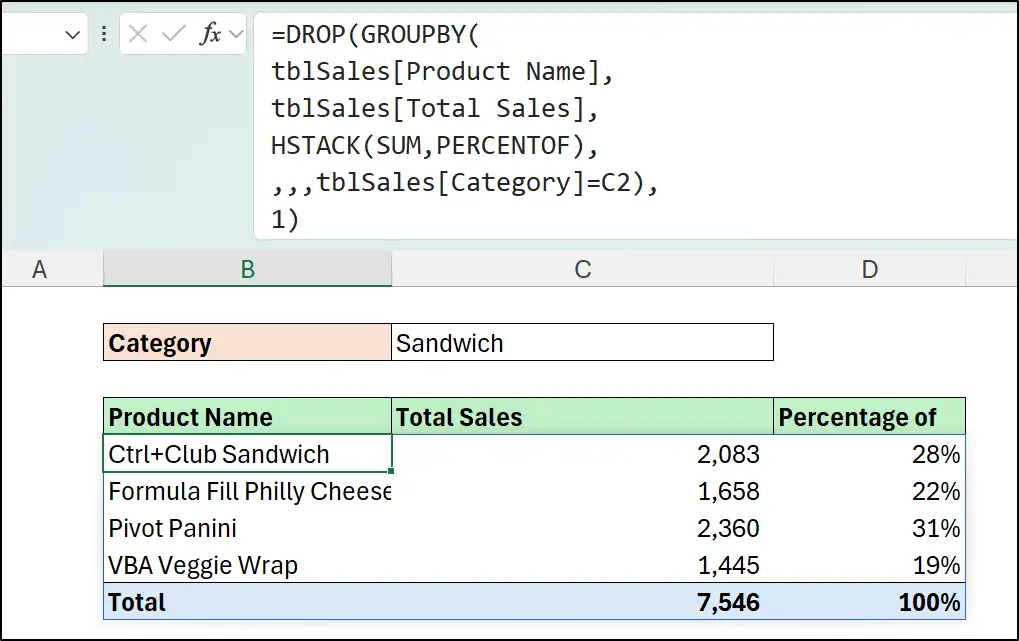
In this example of using multiple aggregations with GROUPBY, you can see that row headers have been shown by default for the SUM and PERCENTOF function columns.
I have my own headers to use for the formula, so will add the DROP function to the formula to remove the first row of GROUPBY results (the column headers.)
=DROP(GROUPBY(
tblSales[Product Name],
tblSales[Total Sales],
HSTACK(SUM,PERCENTOF),
,,,tblSales[Category]=C2),
1)
Summary
The Excel GROUPBY function allows you to create dynamic and interactive summary reports from a single Excel formula.
Using GROUPBY instead of a pivot table report gives more potential when creating charts or in combination with other Excel features such as formulas, checkboxes, drop-down lists, and Slicers.


