See why the Excel pros love the AGGREGATE function. This tutorial will show four examples of the AGGREGATE function in Excel.
By way of a quick introduction, the job of the Excel AGGREGATE function is to perform an aggregation such as sum, average or max on a given range of values and ignore specific rows such those that contain errors, or have been filtered in the range.
Download the practise file to follow along.
Excel AGGREGATE Function
The AGGREGATE function is a really useful function in Excel with a few special powers, which the following examples will focus on highlighting.
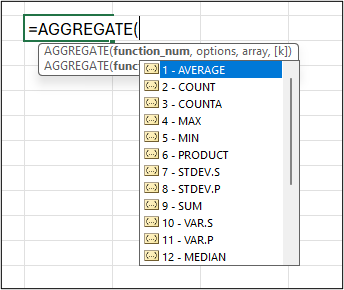
AGGREGATE can execute 19 different Excel functions. This includes popular functions such SUM, COUNT, and AVERAGE, and the likes of MEDIAN, LARGE, and SMALL. Impressive!
It can ignore hidden rows. Typically these are rows that have been filtered. And in this tutorial we will demonstrate this by filtering a table with a Slicer.
AGGREGATE can also ignore rows that contain error values or nested SUBTOTAL and AGGREGATE functions.
The syntax of the Excel AGGREGATE function is as follows.
=AGGREGATE(function_num, options, array, [k])
Function Num: The index number of the function that you want AGGREGATE to execute.
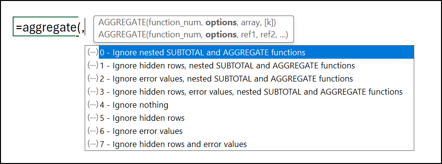
Options: Options such as ignoring error values, hidden rows, and nested subtotal and aggregate functions that can be applied. You can apply a combination of these options, only one of them such as hidden rows, or none at all.
Array: The values that you want to apply the aggregation to.
[k]: An optional argument that can be used with functions such as LARGE and SMALL to specify the kth value, for example the third largest value.
AGGREGATE Function Video
Watch the video to see all examples in action, or read on.
Ignore Subtotals in a Range
The AGGREGATE function is a successor to the SUBTOTAL function of Excel. The SUBTOTAL function can ignore hidden rows and nested subtotal formulas and is still used by Excel today in scenarios such as the total row of Excel tables.
However, it is succeeded by the AGGREGATE function as AGGREGATE brings additional advantages such as ignoring error values and that it can execute a larger list of functions.
In the following data, the SUM function has been used to sum specific ranges. This works, but being this specific with the ranges to sum is time consuming and error prone.
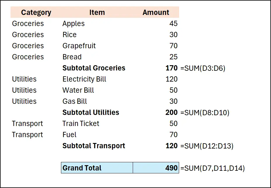
By using the Excel AGGREGATE function to perform the subtotals, instead of sum, we can then use an AGGREGATE formula on the entire range of values. This is because we know that AGGREGATE will ignore any nested subtotals created by the AGGREGATE function (it will not ignore results from a SUM function.)

In this example, the following formula is used for the nested subtotal rows. It uses the SUM function (index 9), ignores the options argument, and then contains the ranges of values to aggregate.
=AGGREGATE(9,,D3:D6)
The following formula is then used for the grand total row. It uses option 3 to ignore everything – hidden rows, error values, and nested SUBTOTAL and AGGREGATE functions. The entire range of values (D3:D14) is then given to sum.
=AGGREGATE(9,3,D3:D14)
Use Slicers with the AGGREGATE Function
Its ability to ignore hidden rows is another top feature of the Excel AGGREGATE function. The best filter tool in Excel is the Slicer, so let’s see an example of AGGREGATE with a Slicer.
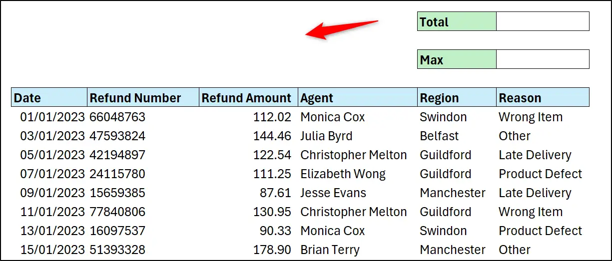
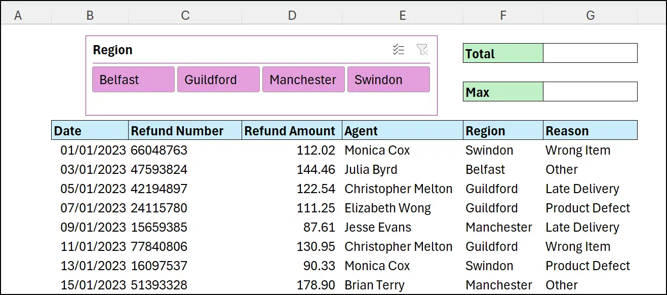
The following table is named tblRefunds. We will add a Slicer for the Region column to filter the data for specific regions. In cells above the table, AGGREGATE will return the filtered total refund amount and the maximum value from the Refund Amount column.
To insert a Slicer, click a cell within the table and click Insert > Slicer. Check the box for the Region column and click OK.
The Slicer can be formatted and resized as required. In this example, the Columns setting on the Slicer tab of the Ribbon is changed to 4 to arrange the region names horizontally instead of vertically.
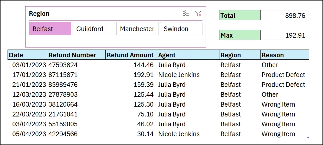
The following AGGREGATE function was used to produce the total value in cell G2. Option 5 has been used to ignore hidden rows only.
=AGGREGATE(9,5,tblRefunds[Refund Amount])
For the maximum value in cell G4, the formula is the same except the use of function number 4 to perform a MAX.
=AGGREGATE(4,5,tblRefunds[Refund Amount])
With the Excel AGGREGATE function the sum and max functions are only aggregating the visible rows. In this example, a filter for the Belfast region is applied by the Slicer.
Create a Function Pick List
With the AGGREGATE functions ability to handle 19 different functions, an interesting use case could be to enable the user to select the function for use from a list.
In the following image, a drop-down list has been added to cell F4 containing the values – Sum, Average, and Max. We will create an AGGREGATE formula that runs the selected function.
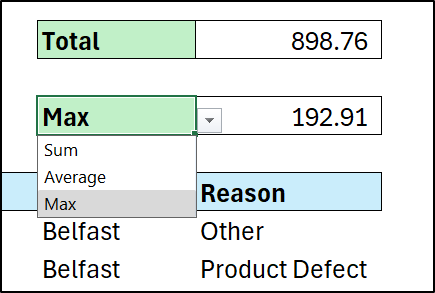
A table (named tblFunctionList) has been created that lists the three values from the drop-down menu (the function names) along with their corresponding aggregate function number. The plan is to use a lookup formula within AGGREGATE to return the requested function number.
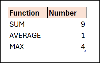
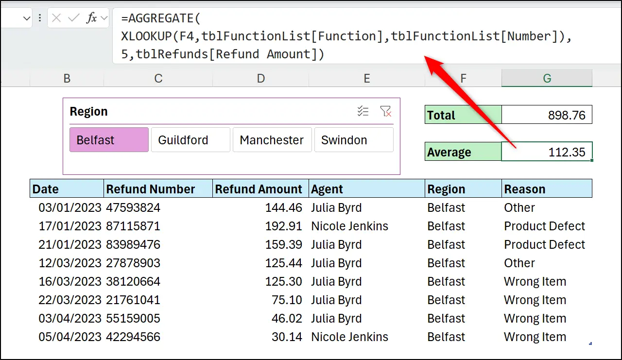
In the following formula, we use the AGGREGATE function with a nested XLOOKUP function to return the results of the selected function. The AVERAGE function has been selected in this example.
=AGGREGATE(
XLOOKUP(F4,tblFunctionList[Function],tblFunctionList[Number]),
5,tblRefunds[Refund Amount])
Connect Slicers to other Formulas
Possibly the sexiest way to use the AGGREGATE function in Excel is to create a connection between Slicers and other Excel formulas. This enables formulas such as FILTER, SUMIFS and more to work on tables filtered by a Slicer.
First, we have added a new column to the table using the following formula. This formula has been used to identify the visible rows of a filtered table.
=AGGREGATE(3,5,[@[Refund Number]])
This AGGREGATE function uses the COUNTA function (function number 3) to count the number of times this Refund Number occurs within the filtered table. Notice the @ symbol used to count only this refund number, not all refund numbers. Option 5 is deployed to ignore hidden rows in the count.
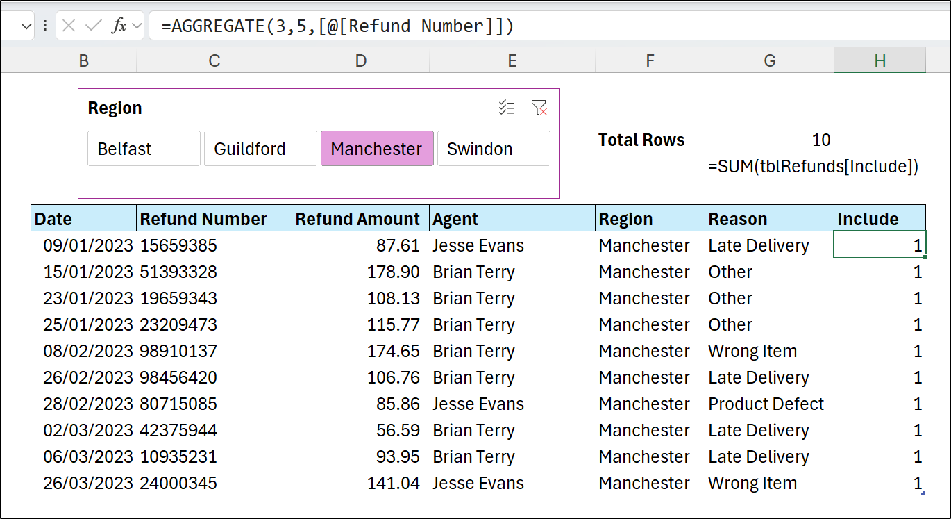
In cell G3 of the image, you can see a sum formula summing the values of the Include column. The result is 10, the number of visible rows. This is confirmation that all hidden rows must be returning 0.
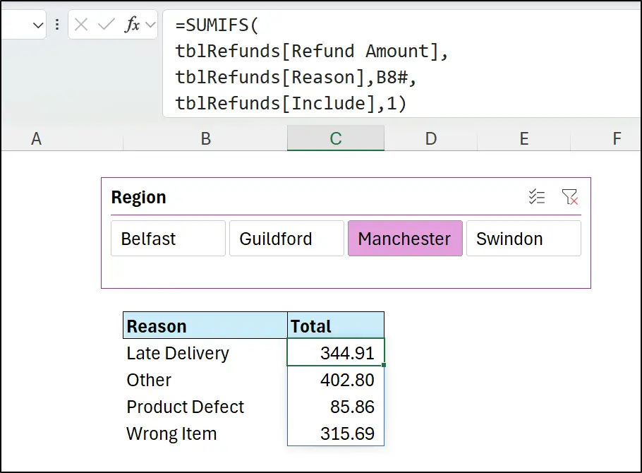
With this Include column, we can now use the condition of the Include column being equal to 1 (the row is visible) in our chosen formula. In this example, that is a SUMIFS function.
=SUMIFS(
tblRefunds[Refund Amount],
tblRefunds[Reason],B8#,
tblRefunds[Include],1)
The SUMIFS is working with the condition applied by the Slicer for the region of Manchester (using the fact that the Include column must be equal to 1) and the condition that the Reason is equal to the value in the spill range of cell B8.
Summary
The Excel AGGREGATE function is a special function with unique qualities, such as to sum values of visible rows only, or to average values while ignoring error values and any nested SUBTOTAL and AGGREGATE functions.
Its ability to allow other formulas to work with a Slicer make it a very special modern Excel function that is highly valued by Excel pros.


