The most commonly used Excel function is SUM. The purpose of the SUM function is to add up all numbers in a range.
In this tutorial, we will see examples of utilising the Excel SUM function to cater for different ‘real world’ scenarios.
Download the practise workbook to follow along.
How to Use SUM in Excel?
Let’s begin with simple examples of using the SUM function to sum values in Excel.
The typical steps to use the SUM function in Excel are as follows.
Click the cell where you wish the total to appear. In this example, that is directly below the values to be summed.
Click the AutoSum button on the Home tab of the Ribbon.
A formula that uses the SUM function appears in the cell. This formula will attempt to identify the range to be summed. This range is shown by a dotted line around the cells Excel thinks you want to use. If the range is not correct, select a different range.
Press Enter.
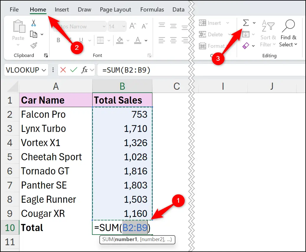
The total appears in the cell. The SUM function will automatically update when any of the numbers change.
Automatically Sum New Rows
A common scenario is that you will need the SUM function to automatically include new values that are added to the bottom of the range.
The two main techniques for this scenario, are to sum the entire column, or to format a range as a table.
To sum the whole column, you can click the Sum button or type =SUM( to begin the formula, then click the column header on the sheet, and press Enter.
The following SUM function adds all values in column B.
=SUM(B:B)
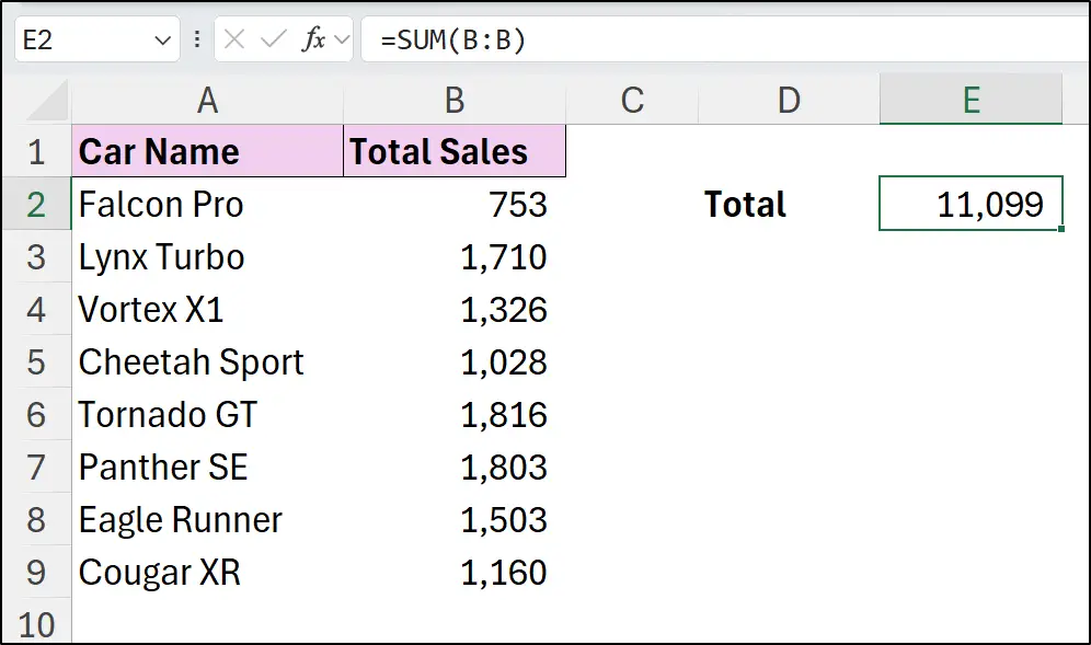
When using this approach, ensure that the formula is not in the same column that you are summing. In this example, that is column B.
This technique is great, as long as you definitely want to sum all values in column B. Be sure that the column only contains numbers that are to be summed.
A superior approach is to format the range as a table, and refer to the Table column instead of the sheet column.
The following formula uses the SUM function on the ‘Total Sales’ column of a table named ‘tblCarSales’.
=SUM(tblCarSales[Total Sales]
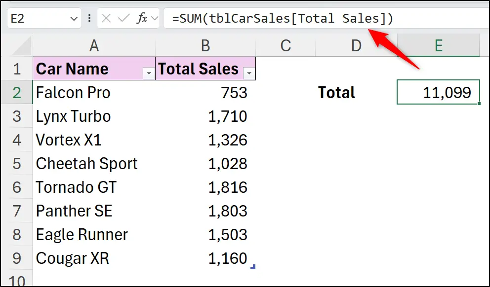
Learning how to use Tables in Excel and why you should is beyond the scope of this tutorial. But right now, the advantage of their use is that when new rows are added to the table, the SUM function in Excel will automatically include them.
Quick SUM Formula Trick for Multiple Sums
If you need to use the SUM function in multiple cells quickly, such as for a matrix of results, this can be done faster than entering the formulas separately.
Take the following example, we have a range of data with values for multiple products and for two years. We need to add all values and return totals down column D and and in cells B10 and C10.
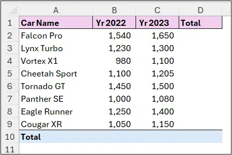
This can be achieved very quickly by selecting the range B2:D10 (the values and the empty cells for the results) and pressing the AutoSum button or pressing the Alt + = shortcut.
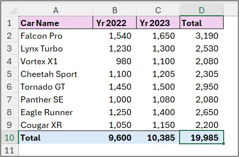
Sum formulas are entered in all empty cells down column D and cell references B10 and C10.
Sum Numbers in Excel on another Sheet
You can use the SUM function to sum numbers from other worksheets in Excel. This is very easy to do (and even easier if you use Tables.)
To use the SUM function on other worksheets.
Start the formula by clicking the AutoSum button or typing =SUM(.
Click on the sheet tab for the worksheet that contains the number to use.
Select the range of values.
Press Enter.
The most common mistake that occurs in my Excel classes is that users click somewhere before they press Enter. Be sure to press Enter immediately after selecting the range of values.
In the following formula, the SUM function adds values in column B of a sheet named ‘Basic Sum’. The single quotations are used in the formula because the sheet name contains a space, and the exclamation mark separates the sheet name from the range.
=SUM('Basic SUM'!B:B)
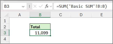
If tables are being used to structure data, the formula would look no different to our first SUM function example. This is another benefit to the use of tables. The fact that their references are meaningful – column B versus ‘Total Sales’.
=SUM(tblCarSales[Total Sales])
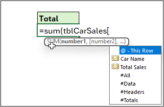
When typing the formula, when entering the table name followed by the opening square bracket, Excel lists the columns (and other table elements) of the table for you to select from. I love this feature of Excel.
Sum Multiple Ranges in Excel
The SUM function can handle up to 255 ranges to sum (far more than you will ever need).
To sum multiple ranges of numbers, simply separate each range with a comma.
In this formula, the SUM function adds the values of cell ranges from two different worksheets – Cambridge and Hull.
=SUM(Cambridge!B2:B9,Hull!C3:C10)
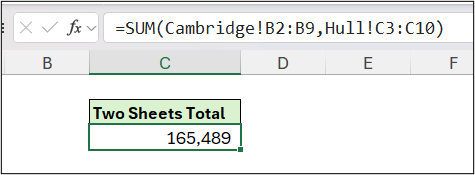
Of course, tables could have been used over standard cell references on a sheet, but it’s nice to mix up the examples.
Create a Cumulative Sum Formula
A common use case for the SUM formula is to create a cumulative sum, otherwise known as a running total.
The technique for a cumulative sum relies on the understanding of relative and absolute references. In this example, we want to sum the values in B2:B13 in a cumulative way, so B2:B3, then B2:B4, then B2:B5, and so on.
To do this, the following SUM function uses an absolute reference for cell B2, which means it does not change when a formula is copied, and a relative reference for cell B3.
=SUM($B$2:B3)
When the formula is copied down, the reference to B3 keeps expanding to the next row automatically, finishing in cell B13.
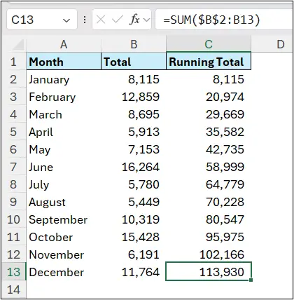
Excel is so awesome, it has a button to write this formula for you.
You can select the range of numbers to create a running total for (in this example that is B2:B13.) Click the Quick Analysis button, click Totals, and scroll across to the right to see the button for Running Totals.
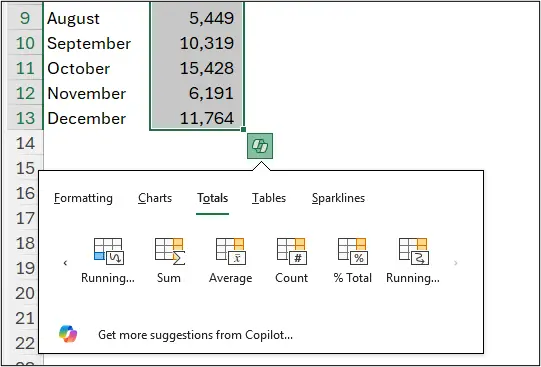
Excel will write the same SUM formula that we wrote previously. Nifty!
It is great to have the knowledge to know how to do this ourselves and not rely on built-in Excel functionality though. Especially if anything was to go wrong in the future. Excel skills to pay the bills.
Advanced Excel SUM Function Examples
The SUM function in Excel is capable of far more than what many users realise.
It can evaluate conditions, handle arrays and other functions such as XLOOKUP can be used to create dynamic range references.
These advanced sum examples are tales for another time, but lets see a little example of SUM being used to sum the products of two columns.
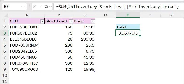
In a situation when you have a column named ‘Stock Level’ and a column named ‘Price’ and the goal is to find the total stock value, users would calculate the stock value for each row (each item) first being summing that column.
If that column is not required for other tasks, and especially if the table has many rows, it can be beneficial to do this all in one Excel formula (if you have 5,000 item rows it would otherwise be 5,001 formulas.)
The following formula multiplies the corresponding values of each column and then sums the results in a single beautiful SUM function.
=SUM(tblInventory[Stock Level]*tblInventory[Price])
