The Excel VLOOKUP function searches for a value in a list and returns information from another column, but the same row to that value. For example, it can search for a reference number and return the price associated to that reference, or search for an employee name and return their start date.
VLOOKUP stands for Vertical Lookup. It gets this name because it looks down columns. You would be right to assume that there is also a HLOOKUP that looks along rows.
The VLOOKUP function is commonly used to consolidate data from multiple sheets, or to compare lists for items that may be missing or match.
Excel VLOOKUP Function Syntax
VLOOKUP requires 4 items of information (arguments) to work.
=VLOOKUP(lookup_value,table_array,col_index_num,[range_lookup])Lookup value – The value that you are looking for. This value can be a number, date or text.
Table array – The table to search for the value in. It looks for the value in the leftmost column of the table.
Col index num – This is the column number of the lookup table that contains the information to return.
Range lookup – Logical value that could be TRUE or FALSE. Are you looking in ranges of values, or for a specific value. VLOOKUP is normally used to find a unique ID
This is an optional argument that if untouched is set to TRUE. This requires the table to be sorted by the leftmost column in ascending order. If the value is not found in the column then the closest match is returned.
If set to FALSE, the data list can remain unsorted and an exact match is returned. If the value is not found a #N/A error message is returned.
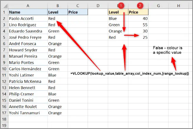
The image below illustrates the role for VLOOKUP. There is a list of members and their membership level. The VLOOKUP looks for the members level in the price list table in columns E and F and returns the price from the second column.

VLOOKUP Function in Excel Example
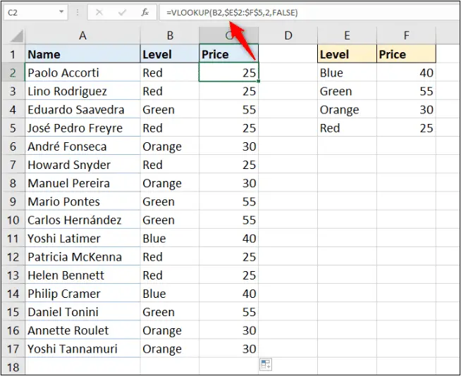
Let’s use the VLOOKUP explained in the image and return the price for each member in the list.
Download the vlookup.xlsx workbook to follow along.
This is the VLOOKUP function to use in cell C2. It can then be copied to the other cells in column C.
=VLOOKUP(B2,$E$2:$F$5,2,FALSE)

This is the most common use of VLOOKUP. To look for a specific value (membership level in this example) in a list and return a value associated with it (the price).
There are loads of scenarios where this behaviour can be useful. You can see different VLOOKUP examples in the video below.
VLOOKUP on other Worksheets and Workbooks
The VLOOKUP function in Excel can look up values in a table on a different worksheet, workbook or named range.
For example, if the lookup table from the previous example (membership price list) was in columns A and B of a different sheet named Memberships. The formula would look like below.
=VLOOKUP(B2,Memberships!$A$2:$B$5,2,FALSE)
And if it was on a sheet named Memberships of a different workbook named Prices 2019, it would look like this.
=VLOOKUP(B2,'[Prices 2019.xlsx]Memberships'!$A$2:$B$5,2,FALSE)
Just be sure that the other workbook is open before you start writing VLOOKUP. You won’t be able to open an Excel file mid formula.
VLOOKUP for a Range Lookup
The VLOOKUP Function can also be used to lookup a value in a range of values. To do this, the last argument of VLOOKUP would be set to True, or omitted.
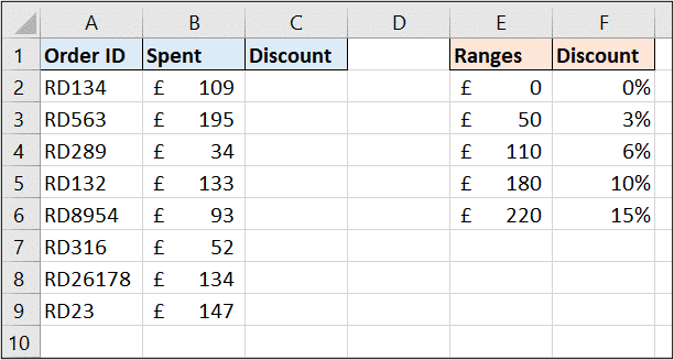
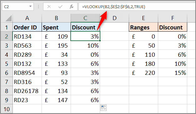
In the example below, we would like to return the discount from column F (second column of the lookup table) dependent upon how much someone has spent.

The following VLOOKUP would do this. It searches for the value in column B down the first column of the lookup table (E) and returns the value from the second column.
=VLOOKUP(B2,$E$2:$F$7,2,True)
When performing range lookups it is essential that the first column of the lookup table is in ascending order. This is not necessary when looking for specific values and setting the last argument to FALSE.


