The UNIQUE function in Excel is a dynamic array formula that returns a distinct or unique list of values from a given array. The array can be a table column, a range of values, or an array returned from another formula.
The syntax of the UNIQUE function is as follows:
UNIQUE(array, [by_col], [exactly_once])- Array: This is the array to return the distinct or unique values from.
- [By _col]: This is an optional argument, and it indicates how to compare; whether by rows or columns. By default, [by_col] is set to FALSE and this returns unique values by rows. To extract unique values by column, set the [by_col] to TRUE.
- [Exactly_once]: An optional argument that returns a unique or distinct list. When set to TRUE, it extracts unique values that appear only once in an array. FALSE will return all distinct values, regardless of how many times they occur in an array.
You can download the sample workbook to follow along.
Return Distinct Values with UNIQUE Function
Consider the following table named tblAttendees, which contains a simple list of names.
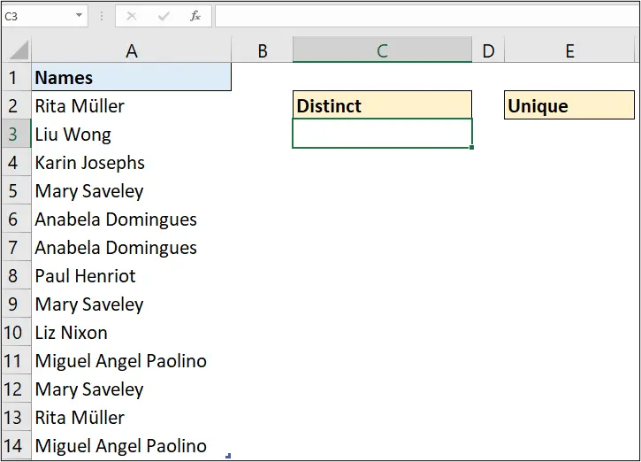
In cell C3, we will return a distinct list of the names in the order they occur within the table using the UNIQUE function in its simplest form.
The formula in cell C3 is written as follows;
=UNIQUE(tblAttendees[Names])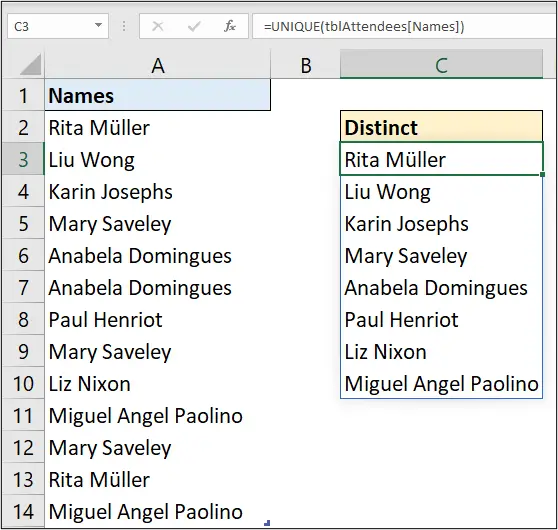
The values returned in cell C3 are a spill range of distinct names that occurred at least once in the tblAttendees table. Only the array was provided to UNIQUE. By default, the Excel UNIQUE function actually returns a distinct list, and not unique (names occur only once).
Return Unique Values with UNIQUE Function
In this second example, we will return a unique list of names to cell E3. These are the names that appear only once in the tblAttendees table.
In the following formula, the UNIQUE function in cell E3 is given the array tblAttendees[Names], the [by_col] argument is skipped, and TRUE was specified for the [exactly_once] argument.
=UNIQUE(tblAttendees[Names],,TRUE)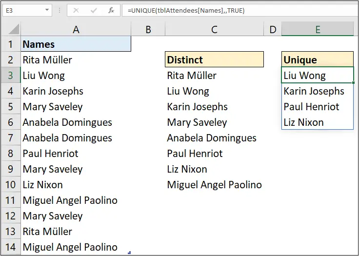
Note: The classic use of the UNIQUE function is similar to using the Remove Duplicates or Advanced Filter feature in Excel to return a distinct list of items from a list. However, as a formula, it is automated. So works great as a source for Data Validation lists and listing distinct values in reports.

Distinct Count Formula with UNIQUE Function
Another great use of the UNIQUE function in Excel is how easy it makes creating a distinct count formula. This is something Excel natively doesn’t have as a worksheet function.
When we wrap the ROWS function around the formula in cell C3, this returns the count of the distinct values in that spill range. The ROWS function literally returns the number of rows in the spill range. An alternative would have been to use the COUNTA function.
The formula is therefore written as follows;
=ROWS(UNIQUE(tblAttendees[Names]))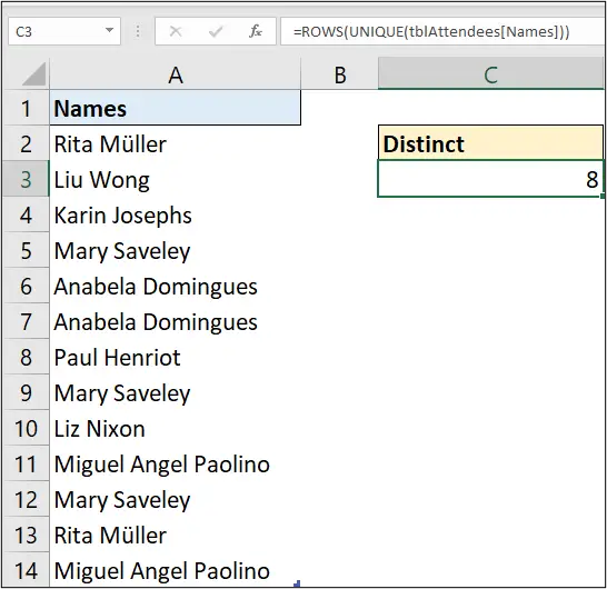
So, although there is no direct distinct count function in the Excel functions list like there is in DAX, or in the Excel data model, the formula is simple thanks to UNIQUE.
Let’s wrap the ROWS function around the formula in cell E3 to return the count of the unique names.
=ROWS(UNIQUE(tblAttendees[Names],,TRUE))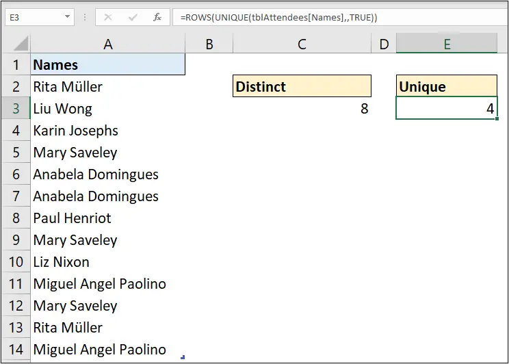
So, there are eight distinct names in the table, and four names that occur once only (are unique).
Compare Columns with the UNIQUE Function
Although it is typical to compare rows with the UNIQUE function, it can also be used to compare columns.
Let’s demonstrate how it’s done using the following range.

The range has names of regions across the header row.
We want to return a distinct list of those region names. The Excel UNIQUE function will be used to return a distinct list to cell B11.
In the following formula, TRUE is entered for the [by_col] argument. This specifies for UNIQUE to compare values across columns rather than the default behaviour of across rows.
=UNIQUE(B2:I2,TRUE)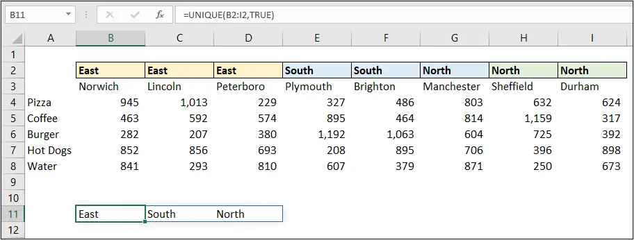
The names of the regions are returned in the same orientation (horizontally) as they appeared in the range. Wrap the TRANSPOSE function around the UNIQUE function to get your result in a vertical range.
=TRANSPOSE(UNIQUE(B2:I2,TRUE))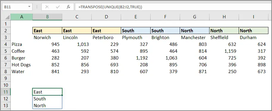
UNIQUE Function as a Source of a Drop-Down List
The UNIQUE function in Excel is commonly used to create a dynamic source for a drop-down list. Let’s see a practical use case for this.
The following table highlighted is named tblSales, and we want a drop-down list in cell G2 of the distinct region names from the [Region] column of the table. This range will be used as an input cell for a dynamic report.
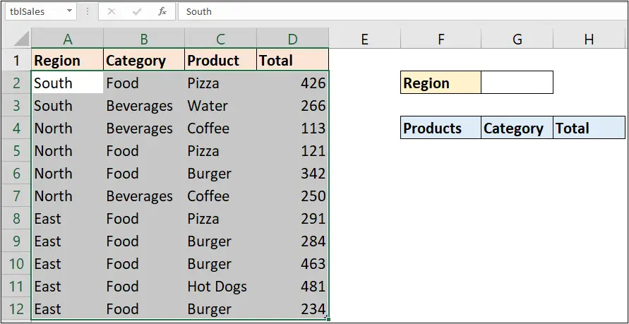
To do this, we first use the UNIQUE function to return a distinct list of those region names in a new sheet named Drop Down.
The following formula is used in cell A2.
=UNIQUE(tblSales[Region])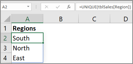
The regions are returned in the order that they appear in the tblSales table.
Wrap the SORT function around the formula to return the regions in ascending order. If someone were to change the order they occur within the tblSales table, it wouldn’t affect the order of the drop-down list.
=SORT(UNIQUE(tblSales[Region]))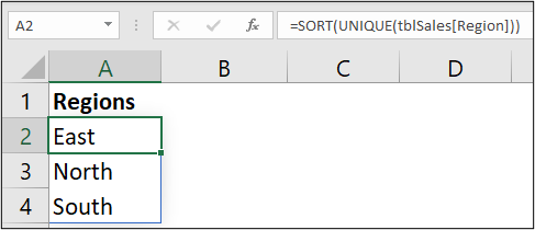
To create the drop-down list;
- Click in cell G2 on the report sheet.
- Click Data > Data Validation.
- Select List from the Allow list.
- Click in the Source box, and click cell A2 of the Drop Down worksheet.
- Type the hash # symbol to append it to the range. The resulting reference will be as follows.
='Drop Down'!$A$2#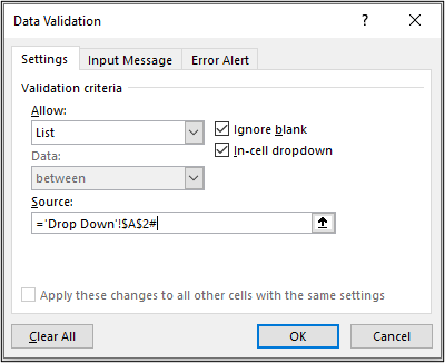
Click OK to close the Data Validation window.
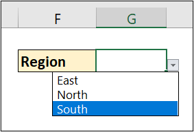
Cell G2 now contains a drop-down list that will be used as an input cell for our dynamic report. This list is dynamic, and if more regions are added to tblSales, the drop-down will pick them up and they will be ordered correctly.
Note: The # symbol is the spill range operator, and it indicates that the rest of the cells in the spill range are selected as well.
Distinct List of Values for Pivot Style Report
The UNIQUE function in Excel is great for helping create pivot style reports as an alternative to the fantastic PivotTables in Excel. It is used to generate the dynamic row or column labels for the report.
In cell F5, the following formula is used to create a distinct list of products for the row labels of the report. You are getting very familiar with this combination of the SORT and UNIQUE functions. It is so useful.
=SORT(UNIQUE(tblSales[Product]))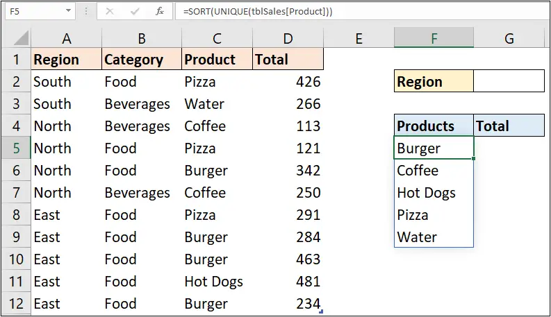
To return the total for each product in the spill range, the Excel SUMIFS function is used. The # symbol is used to connect the criteria argument to the F5 spill range.
=SUMIFS(tblSales[Total],tblSales[Product],F5#)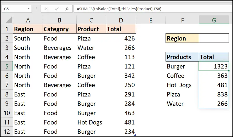
Return Multiple Columns with the UNIQUE Function
All examples of the Excel UNIQUE function so far have returned a single column from a table. In this example, we will return specific columns and in a specific order.
In cell F5, the following formula returns the distinct values from the [Product] and [Category] columns in that order. This is done using the CHOOSECOLS function and specifying the return of column 3 and then 2 from tblSales.
The SORT function sorts the results in ascending order by the second column of the array (the category column).
=SORT(UNIQUE(CHOOSECOLS(tblSales,3,2)),2)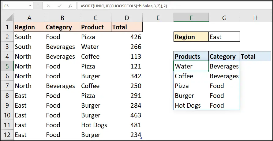
This relatively new function in Excel makes it easy to choose specific columns from a table or array.
Please note that in the tblSales table, the [Category] column precedes the [Product] column. While in our report range, the [Products] precede our [Category]. This is a deliberate act to simply show what can be done.
To produce the [Total] column in cell H5, the CHOOSECOLS function was used with the SUMIFS function. This is because the spill range returned with the UNIQUE formula is two columns wide, and the “criteria1” argument of SUMIFS demands the first column of the spill range only.
=SUMIFS(tblSales[Total],tblSales[Product],CHOOSECOLS(F5#,1))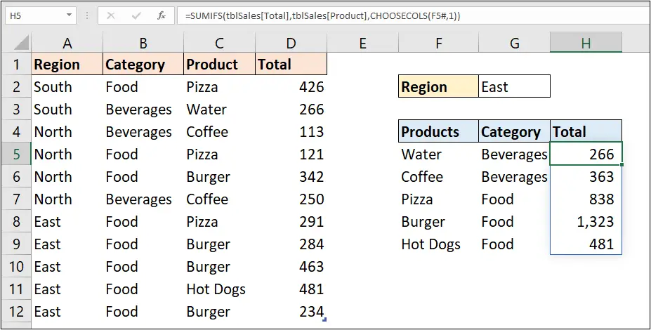
Add the Report Filter
To complete this dynamic report example, we need to include the drop-down list that was created in cell G2, so that the report can be filtered for a specific region.
In the following formula, the Excel FILTER function was added to filter the [Region] column for the value in cell G2.
=SORT(UNIQUE(
CHOOSECOLS(FILTER(tblSales,tblSales[Region]=G2),3,2),
),2)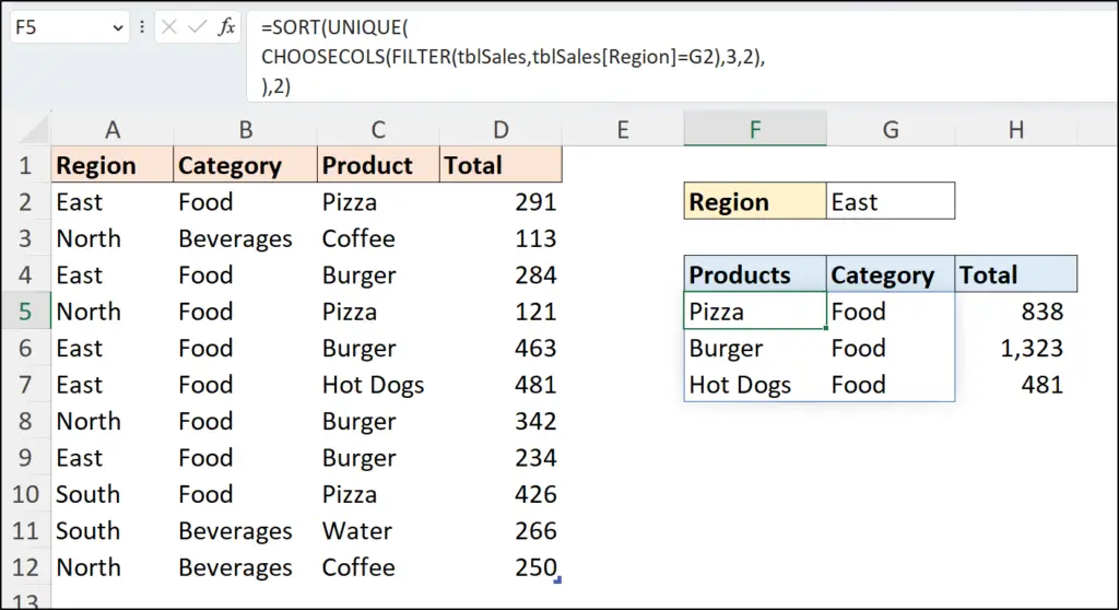
UNIQUE in Excel is a tremendous function and has become a firm favourite for many Excel users.
Do you love the UNIQUE function?


