The Excel SUMPRODUCT function is a hidden gem. The purpose of the SUMPRODUCT function is to return the sum of products from 1 or more arrays. Now this may not sound that useful, but let me explain further.
It’s syntax is:
=SUMPRODUCT(array1, [array2], [array3], ...)
The Excel SUMPRODUCT function works by multiplying a group of numbers and then adding the results. Each array of SUMPRODUCT is a range of values. These arrays must be of the same dimension.
SUMPRODUCT Function Example
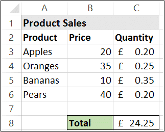
The SUMPRODUCT formula below has been used to total the sales of fruit. This has been achieved in one formula instead of multiplying each sales quantity by its price in a column, and then summing the results.
=SUMPRODUCT(B3:B6,C3:C6)

The formula first multiplies the values of each array e.g. 20*0.2 & 35*0.25 & 10*0.35 & 40* 0.2. These products of 4, 8.75, 3.5 and 8 are then summed to return the results of 24.25.
However Excel users have taken it far beyond its initial design. The SUMPRODUCT function can normally be found performing powerful array calculations on user’s spreadsheets.
Complex Summing and Counting Formulas
The Excel SUMPRODUCT function can be used as an alternative to functions such as SUMIFS and COUNTIFS to perform complex summing and counting formulas.
The benefit of using SUMPRODUCT is that it can be an easier way of incorporating different conditional logic into the formula.
The COUNTIFS function uses the AND logic between each condition. To apply OR logic, you would need to add two different COUNTIFS functions together. However, with SUMPRODUCT the criteria can all be written within the same formula.
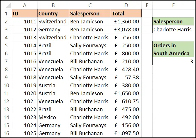
The formula below has been used in cell F7 to perform a complex count.
=SUMPRODUCT(((B2:B16="Venezuela")+(B2:B16="Brazil"))*(C2:C16=F3))
In this example, you can think of the “+” operator is being used to apply OR logic, and then the “*” operator for AND logic. It ultimately counts the number of orders from Venezuela OR Brazil AND were taken by the salesperson in cell F3.

The formula below includes an additional array for the values in D2:D16. This will return a sum of the orders, instead of the count from the previous example.
=SUMPRODUCT(((B2:B16="Venezuela")+(B2:B16="Brazil"))*(C2:C16=F3)*(D2:D16))
Summing Every Nth Row
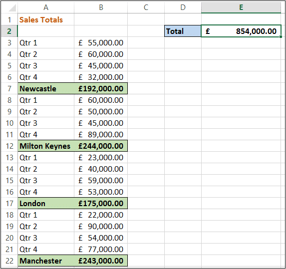
In an example when the values to sum are not in consecutive cells, the Excel SUMPRODUCT function can come in useful. Lets imagine a scenario when they are in every 5th row like in the image below.

The formula below has been entered into cell E2 to sum the values for each region in column B.
=SUMPRODUCT((MOD(ROW($B$3:$B$22)-2,5)=0)*($B$3:$B$22))
The ROW function is used to return the row number of the current value. 2 is subtracted from this row number because in this example the list starts from row 3, so the 5th row in the range is row 7. The value to be added is always 2 cells above the multiples of 5 (5, 10, 15 and 20).
The MOD function is used to divide the row number by 5 to determine if it is the 5th cell. MOD will result in 0 if it is the 5th row, so the SUMPRODUCT function tests if it is equal to 0.
SUMPRODUCT then multiplies the result (which will be 1 if it is the 5th cell) with the value of the cell. All the values that meet the condition are then summed.


