The SUMIFS function in Excel is one of the most useful functions in Excel. I absolutely love it!
In this tutorial, we will see five examples of using the SUMIFS function.
Download the workbook used in the tutorial to follow along and practise.
Introduction to the SUMIFS Function
The SUMIFS function in Excel will sum values based on one or multiple criteria being met.
There is also a SUMIF function Excel. This only handles one criteria, so was effectively replaced by SUMIFS back in 2007. SUMIF is still used heavily to this day however.
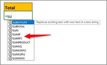
The SUMIFS function requires three pieces of information – the sum range, the criteria range and the criteria.
The sum range is provided first, and then followed by up to 127 (nobody needs that many) criteria range and criteria pairs.
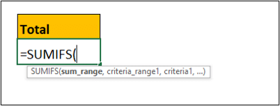
- Sum range: The range of values to be summed.
- Criteria range 1: The range to be tested using criteria 1. If the criteria is met, the corresponding value from the sum range is included in the sum.
- Criteria 1: The criteria to evaluate in criteria range 1. This can be entered as a string, a number or an expression. The following are all valid ways to enter the criteria; “complete”, D4, 23, “>=25” and “>=”&D4.
- [Criteria range 2], [criteria 2]: Additional associated criteria ranges and criteria for testing multiple conditions.
Let’s get into these SUMIFS function examples.
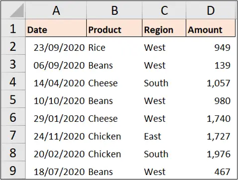
For each example, we will be using the data shown below. This is just a snapshot of the full table of data to get a feel for it.
This range has been formatted as a table named Sales.

Example 1: SUMIFS with One Text Condition
In this first example, we want to sum the values from the Amount column, only for the product “Cheese.”
The following formula has been entered into cell F6.
=SUMIFS(Sales[Amount],Sales[Product],"Cheese")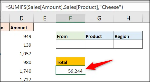
In this example, the text value being used for the criteria has been ‘hard coded’ into the formula. To do this, it has been enclosed in the double quotation marks.
Example 2: Use a Cell Value for Dynamic Criteria
In this example, we will make a slight change from the previous formula, and use a cell value for the criteria instead of writing it directly into the formula.
The product we will use for the criteria has been entered into cell G3 of the worksheet.
=SUMIFS(Sales[Amount],Sales[Product],G3)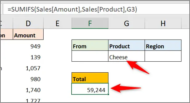
Example 3: SUMIFS Function with Multiple Criteria
In this next example, we will use the SUMIFS function in Excel with multiple criteria.
We want to sum the values from the Amount column, where the Product meets the value in cell G3 and the Region meets the product entered into cell H3.
=SUMIFS(Sales[Amount],Sales[Product],G3,Sales[Region],H3)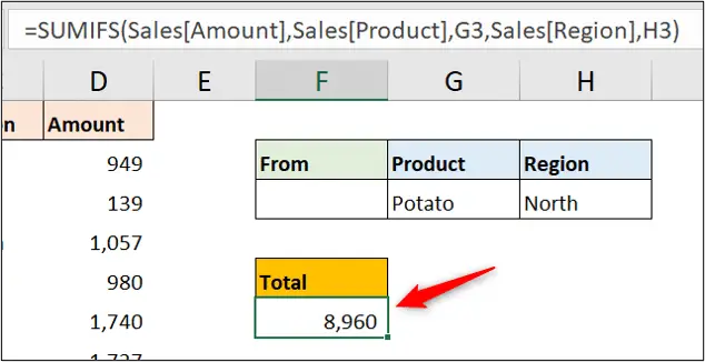
You can see how easy the SUMIFS function makes this. You can enter as many conditions as you require by simply repeating the criteria range and criteria pairs.
Example 4: Test Numeric Values with the SUMIFS Function in Excel
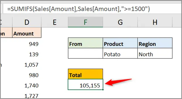
Let’s now see an example of testing a numeric value with SUMIFS.
We want to sum the values, only for the orders that have an Amount of 1500 or more.
For this, we need to include the logical operators “>=”. Because these are text characters, we will enter the whole criteria as text.
=SUMIFS(Sales[Amount],Sales[Amount],">=1500")The Amount column has been used for both the sum range and the criteria range, in this example.
Example 5: Combine Text and a Cell Value for SUMIFS Criteria
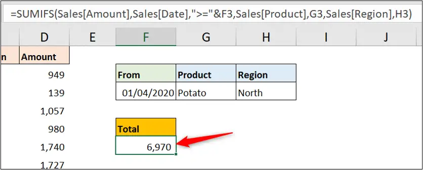
For this final SUMIFS function example, we will bring it all together and use three conditions in our formula. We also want to combine text and a cell value for one of the criteria.
We want to sum the values if the Date is the greater than or equal to the one entered into cell F3, the Product meets the value entered into cell G3, and the Region meets the value entered into cell H3.
This example required combining the “>=” operators with the value of cell F3, so that the date used for the criteria is dynamic. This was done by using the ampersand “&” e.g., “>=”&F3.
This technique is great when testing numeric values with SUMIFS. In the previous example, we entered “>=1500” into the formula as a constant.
=SUMIFS(Sales[Amount],Sales[Date],">="&F3,Sales[Product],G3,Sales[Region],H3)
The SUMIFS function in Excel is absolutely fantastic. I love the fact that it is very powerful and very useful, yet also easy to use.
See Also
- The excellent SUMPRODUCT function
- FILTER function – is this the best Excel function
- The power of Merge Queries in Excel


