The INDEX function in Excel can lookup and return a value, array of values or a range. It is a very powerful and useful Excel function. For me, it is probably the best function in Excel.
One of the biggest strengths of the Excel INDEX function is its versatility. It returns values or a reference from a given row and column. When combined with other functions, this is massive.
This tutorial will demonstrate multiple INDEX function examples to showcase the different abilities of this wonderful function.
Excel INDEX Function Anatomy
The INDEX function in Excel has two different syntaxes.

The Excel INDEX function is most commonly used with the first syntax. All of the INDEX function examples in this tutorial will follow that syntax, except the final example.
- Array – A range or array from which to return values or a reference.
- Row num – The row number in the array from which to return the values or reference. If omitted, a column number must be given.
- Column num – The column number in the array from which to return the values or reference. If omitted, a row number must be given.
Download the sample Excel workbook to practise the INDEX function examples.
Basics of the INDEX Function in Excel
The INDEX function is most commonly used to lookup and return a value. The formula below is entered into cell G3 and is returning the sales value for pizza. This value is in the 3rd row and the 3rd column of the range B3:D7.
=INDEX($B$3:$D$7,3,3)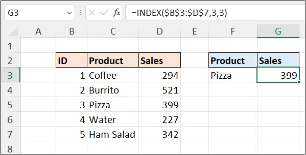
Notice that the INDEX function is returning the value from the 3rd row and 3rd column from the given range, not the 3rd row and 3rd column of the worksheet.
INDEX and MATCH Lookup Formula
The most common use of INDEX, is to be used along with the MATCH function for a powerful lookup formula.
In the previous example, the row and column number were entered as constants. This is not a practical use of INDEX. The row and/or column numbers are normally returned by some other function, or even a form control.
MATCH is the most common function used to assist INDEX with this task.
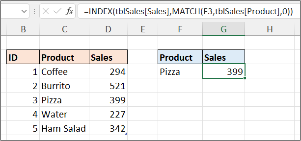
To return the sales of pizza, as in the previous example, the following INDEX and MATCH formula could be used.
In the formula this time, the array has been formatted as a table named tblSales. Tables are much easier and more meaningful as formula references compared to typical range references.
=INDEX(tblSales[Sales],MATCH(F3,tblSales[Product],0))The MATCH function returns the row number of pizza (cell F3) in the Product column and passes it to INDEX. Notice that the column number is omitted as the array INDEX is using is only one column wide (the Sales column).
Two-Way Lookup with INDEX and MATCH
If we needed to provide a column number also, another MATCH function can be used to return the column number.
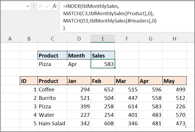
In the following formula, INDEX has been given the entire table (named tblMonthlySales) as the array to use.
One MATCH function is used to return the row number of the product in cell C3, and another MATCH function is returning the column number of the month entered in cell D3, along the table header row.
=INDEX(tblMonthlySales,
MATCH(C3,tblMonthlySales[Product],0),
MATCH(D3,tblMonthlySales[#Headers],0)
)
The formula has been broken over multiple lines to make it easier to read. This is done by pressing Alt + Enter.
Return the Last Value in a Column or Row
The INDEX function in Excel is perfect for retrieving values from a relative position, for example, the last row or column in a table.
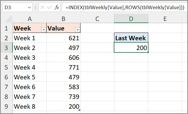
In the following formula, the INDEX function is returning the last value in the Value column of a table named tblWeekly.
=INDEX(tblWeekly[Value],ROWS(tblWeekly[Value]))The ROWS function is used to return the number of rows in the tblWeekly table. This is provided to INDEX as the row number to retrieve the value from. The COUNT and COUNTA functions are often used for this task also.
Return an Array of Values with the Excel INDEX Function
If an array has more than one row and column, and only a row number or column number is provided, then INDEX returns all the values from that row or column in the array.
This functionality is awesome. It can be used to feed another function or given to a chart to be used.
In the following formula, the SUM function totals the values for the last column in a table named tblProductSales.
=SUM(INDEX(tblProductSales,,COLUMNS(tblProductSales)))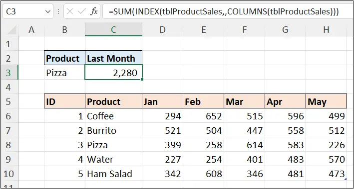
The following formula shows only the INDEX function part of the formula.
=INDEX(tblProductSales,,COLUMNS(tblProductSales))The INDEX function is using the entire table of tblProductSales as its array to return from. The row index num argument is omitted, so INDEX returns the values from all rows of the table. The COLUMNS function returns the last column number in the table.
So, the INDEX function returns the values {499; 512; 226; 570; 473} to be summed.
INDEX Function in Excel to Return a Range
One of the great strengths of the Excel INDEX function is its ability to return a range. There are only a few functions in Excel that can do this, such as XLOOKUP, INDIRECT and OFFSET and a few others. Notably, the most famous lookup function in Excel – VLOOKUP, cannot perform this task.
In this example, we will use the INDEX function to create a dynamic range that we will use as the source for a Data Validation list.
The following image shows a list of countries that begin in cell A2. In cell C2, there is a Data Validation list.
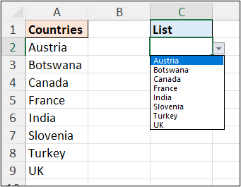
To ensure that the Data Validation list automatically updates when countries are added and removed from the list, INDEX is used to create a dynamic range.
The following formula is used. A2 is specified as the start cell and then the range operator, the colon “:”, is entered. INDEX is then added along with COUNTA to return the reference of the last used cell in column A.
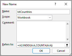
=A2:INDEX(A:A,COUNTA(A:A))Now, this formula cannot be entered directly into the Data Validation rule, so a name is defined using the formula first.
Click Formulas > Define Name to open the New Name window. lstCountries is entered as the name and the formula is pasted in the Refers to box.
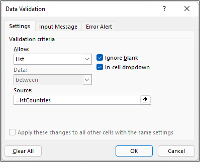
The Data validation list and then be created using this name as its source.
Click Data > Data Validation to open the Data Validation window. Select List from the Allow list and enter =lstCountries for the Source.
Excel INDEX Function to Choose a Range
For the final Excel INDEX function example, we will use the INDEX function to return a range from a list of options. The range that is chosen, will be specified by a cell value.
Now, it is cool that the INDEX function can do this, and it is included in this tutorial for completeness. However, functions such as SWITCH, INDIRECT and CHOOSE are better choices for this task.
One limitation for INDEX is that the range must be on the same worksheet.
For this example, we will be using the second syntax of the INDEX function in Excel.
=INDEX(reference, row_num, [column_num], [area_num])
- Reference – This is a reference to one or more ranges
- Row num – The row number in a given array or range from which to return a value or a reference. If omitted, a column number must be provided.
- Column num – The column number in a given array or range from which to return a value or a reference. If omitted, a row number must be provided.
- Area num – The index number of the range from the Reference argument that you want to return.
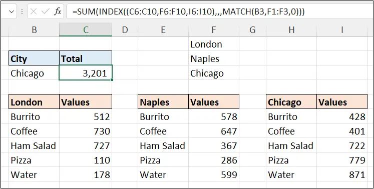
In the following formula, the SUM function is used to sum the values in the range returned by INDEX. The INDEX function has a reference list of three ranges – C6:C10, F6:F10 and I6:I10. These relate to the cities of London, Naples and Chicago, in that order.
=SUM(INDEX((C6:C10,F6:F10,I6:I10),,,MATCH(B3,F1:F3,0)))The row and column index number arguments are omitted. The MATCH function is used to return the index number of the required range. It searches for the city name in cell B3 down the range of values in F1:F3 (this did not need to be on the same sheet, but was done so for easier understanding).
