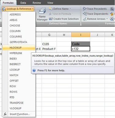
Hlookup works in the same way as Vlookup except that it searches for a value in the top row of a table and returns a value from a specified row.
=Hlookup(lookup_value,table_array,row_index_num,[range_lookup])
As with Vlookup, if range lookup is omitted or set to true the top row of values must be sorted in ascending order. Set range lookup to false for an exact match.
Let’s run a Hlookup on the stock sheet below in cell I6. When a code is entered into cell I3 the stock level will automatically appear in cell I6 as a result of the function.
Download the Stock Sheet hlookup workbook to follow along.

Select cell I6
Click the Formulas tab, and then Lookup and Reference from the Function Library. Select Hlookup from the list.
Once you get used to writing functions you may find it quicker and easier to type them directly into the cell.

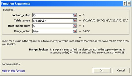
The Arguments dialogue box appears asking for the information the Hlookup needs.
The Lookup value is I3 as this is the cell that holds the value to search for.
The Table array is$A$2:$G$7 as this cell range holds the data list that Hlookup will search in for the value. Hlookup searches in the top row for the value, which in this case is row 2. This range is made absolute.
The Row index num is 5 as the Stock Level row is the 5th row down.
Range lookup is false as we want an exact match.

Click Ok
Type a value in cell I3 to see the HLOOKUP update the cell containing its stock value
Examples of HLOOKUP being used on the stock sheet HLOOKUP workbook.
| Code | Example | Result |
|---|---|---|
| C132 | =Hlookup(I3,$A$2:$G$7,6,false) | £349.30 |
| C134 | =Hlookup(I3,$A$2:$G$7,2) | Product E |
| C138 | =Hlookup(I3,$A$2:$G$7,5) | 18 |
| C134 | =Hlookup(I3,$A$3:$G$7,5,false) | #N/A |


