Using the Excel SORT function, you can sort data in Excel automatically with a formula. This assists us greatly when creating dynamic reports and dashboards without the use of Excel Pivot Tables.
Two of the most commonly used features of Excel are the Sort and Filter buttons on the Data tab of the Ribbon (and elsewhere). Having a formula equivalent of that functionality is a game changer.
In this tutorial, we explain how to use the Excel SORT function and see a few examples of it in action. Download the sample file to follow along.
How to use the SORT Function in Excel
The SORT function in Excel is a dynamic array function used to sort tables, ranges and especially arrays in Excel.
It is awesome for applying a sort order automatically to the results of a formula.
The syntax of the SORT function is as follows.
=SORT(array, [sort_index], [sort_order], [by_col]) What do these arguments mean?
Array: The range, table or array that you want to sort.
Sort Index: The index number that represents the column or row of the array that you want to sort by. If omitted, the first column, or first row, of the array is used.
Sort Order: The order that the column or row should be sorted. Enter 1 to sort in ascending order, or -1 for descending order. If omitted, it will sort in ascending order.
By Col: Do you want to sort by column? By default, FALSE is used meaning that the SORT function will sort by row (vertical sort). Enter TRUE to specify to sort by column (horizontal sort).
We will not demonstrate the fourth argument in this tutorial as sorting horizontally is so rarely used, however, the functionality is duly noted.
There is also a dynamic array function in Excel named SORTBY. The SORTBY function differs from SORT by allowing you to specify the sort column by name instead of an index number, and also enables the sorting by columns outside of the returned array.
Let’s see some examples of the Excel SORT function.
Basic Excel SORT Formula Example
In this example, we have a table named tblStoreSales that contains a store name and a sales value.
The following SORT formula is entered in cell E3 to sort the values by the second column and in descending order.
=SORT(tblStoreSales,2,-1)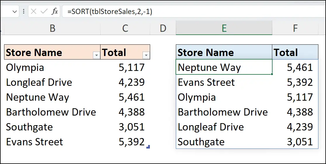
In the formula, the 2 is entered for the sort index to specify that the second column should be used as the column to sort by. And the -1 is entered for the sort order to stipulate descending order as the desired sort direction.
SORT + UNIQUE Formula Example
Combining the SORT and UNIQUE function in Excel is great for dynamically removing duplicates and ordering values all in one Excel formula.
We have the following Excel table named tblSales with a [Product] column that contains duplicate values. We want to return a distinct list of the product names in ascending order to cell E3.
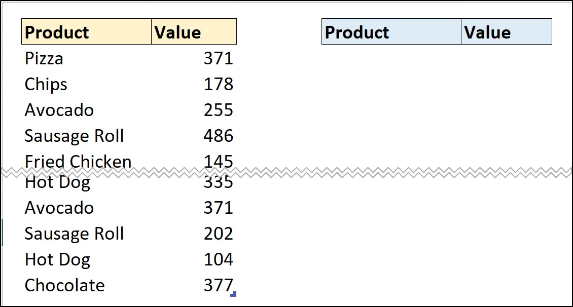
In the following SORT formula, the UNIQUE function returns an array containing the distinct values from the [Product] column of tblSales. The SORT function sorts the values in the array in ascending order.
=SORT(UNIQUE(tblSales[Product]))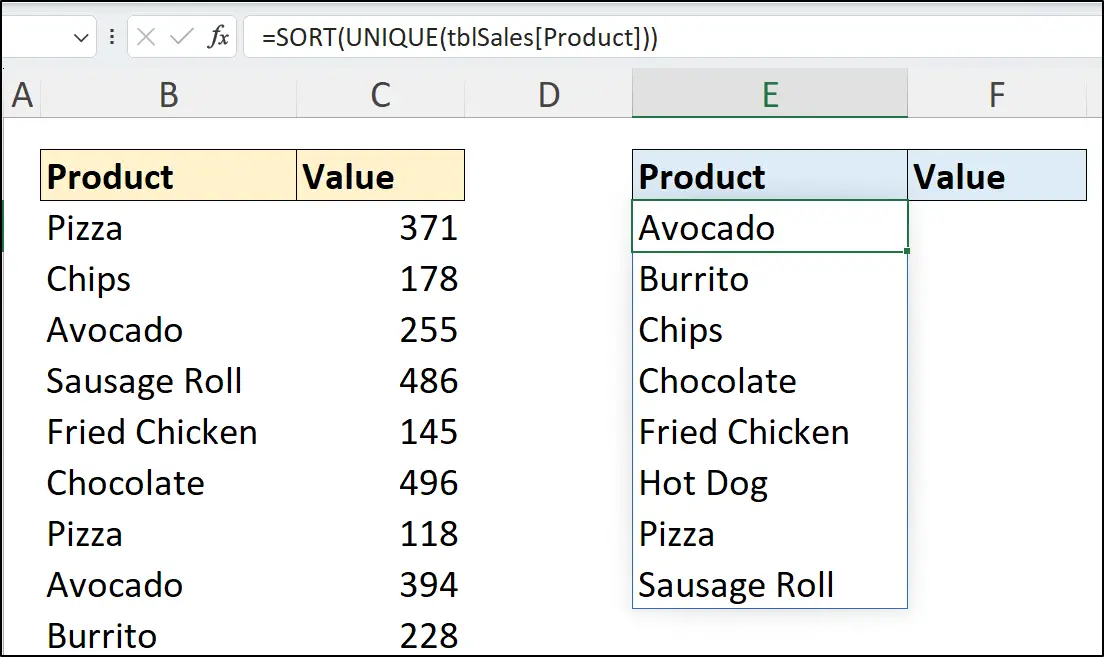
Note that the sort column index number and the order to sort by were not specified in this SORT function. When omitted, 1 is used for the column index, and as this array is only one column wide, this is good. And when the sort order is omitted, ascending order is used.
This has resulted in a spill range containing the distinct list of products in alphabetical order.
The SUMIFS function can then be entered into cell F3 and connected to the spill range from the SORT formula to sum the values for each product.
For the criteria argument of the SUMIFS function, E3# was entered. Cell E3 is the origin cell of the dynamic array formula, and the # sign connects the formula to the spill range. So both Excel formulas will update in sync with each other.
=SUMIFS(tblSales[Value],tblSales[Product],E3#)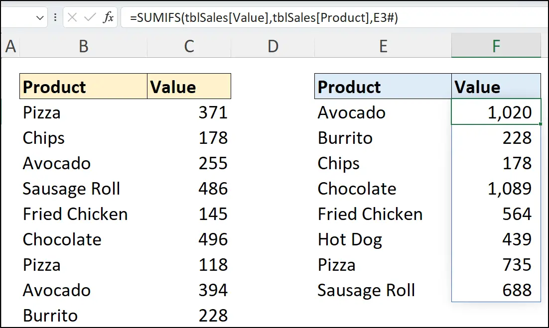
Sorting values returned by another function such as UNIQUE, is a typical application of the Excel SORT function.

Sorting Arrays with the Excel SORT Function
In the last example, the array returned by the UNIQUE function was used by the SORT function as its input. This is the most common use of SORT, to sort an array returned by another function.
So, let’s take this example further and see an advanced example of the SORT function being used in this way.
In this example, we want to improve upon the results of the previous formula, and sort the results by the sum of the product values in descending order (column F). As shown below, the results are currently returned in ascending order by product name (column E).

To do this, we will combine the two arrays (the formulas in cell E3 and F3) into a single array using the HSTACK function in Excel. This function will horizontally stack the two arrays into a single two column array.
We can then sort the second column of this array in descending order.
In the following formula, the SORT function sorts the array returned by the HSTACK function. You can see the 2 and -1 on the end of the formula, specifying to sort the second column and in descending order respectively.
=SORT(HSTACK(
UNIQUE(tblSales[Product]),
SUMIFS(tblSales[Value],tblSales[Product],UNIQUE(tblSales[Product]))
),2,-1)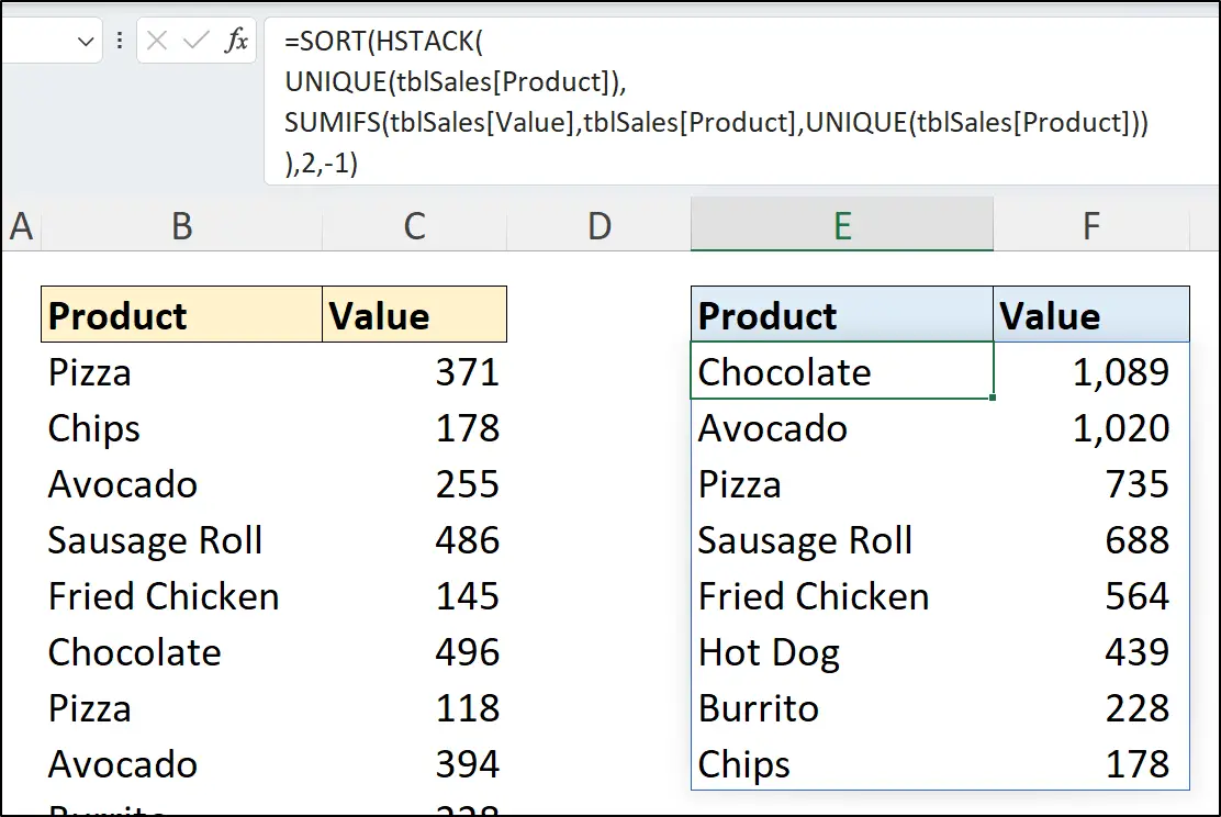
In the SUMIFS part of this formula, the E3# reference from the previous example is replaced by the UNIQUE function. This was necessary because after combining the formulas into one, we no longer had the results in cell E3 to reference.
Sort Multiple Columns with the Excel SORT Function
For the final Excel SORT function example, we will look at how to sort more than one column with the SORT function.
The table we will use, named tblScores, contains a [Name], [Region], and [Score] column. We will use the Excel Sort function to sort by region in ascending order, and then by score in descending order.
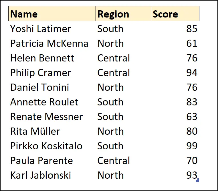
In the following formula, values to specify the sort indexes and order to sort by are entered as array constants. For the sort index, the second column followed by the third column is stated. And for the sort order, ascending and then descending order are stated.
=SORT(tblScores,{2,3},{1,-1})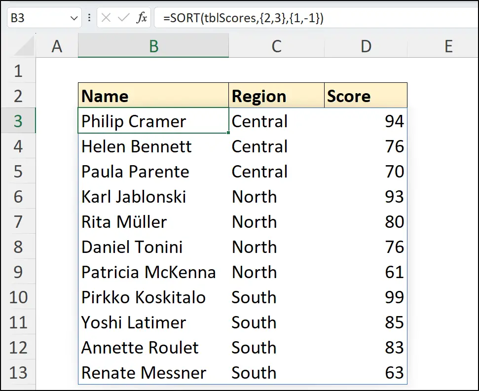
So, although the ability to sort by multiple columns is not natively provided like it is with the SORTBY function, it is easy to apply with array constants.
All examples in this tutorial return arrays that use consecutive columns. Learn how functions such as CHOOSE and CHOOSECOLS can be used to return and sort non-adjacent columns of an array.
Wrap Up
The SORT function in Excel is one of the dynamic array functions and enables us to easily sort the result of a range or array dynamically.
This tutorial demonstrated examples where the SORT function can be combined with other Excel functions to dynamically order the results of arrays.
To learn over 150 Excel functions, pick up a copy of Advanced Excel Formulas. It includes more than 500 formula examples with practise files to follow along.


