Use wildcard characters in Excel formulas to perform partial matches on text. This can be extremely useful. Excel allows the use of wildcards in filters, the Find and Replace tool and especially in formulas.
This blog post explores some examples of using wildcard characters in formulas to find, sum or count cells containing partial matches to what we are searching for.
Watch the Video – Wildcard Characters in Excel Formulas
If you prefer a video tutorial, then check it out below, otherwise please continue for the written tutorial.
Before we look at some examples of wildcard characters in Excel formulas, we should discuss the three types of wildcard characters you can use in Excel.
- * (asterisk) – represents any number of characters. For example, In* could mean India, Indonesia, Indianapolis, Innsbruck.
- ? (question mark) – represents one single character. For example, L?ndon could mean London, or Landon.
- ~ (tilde) – used to identify a wildcard character in the text. For example, if you wanted to find the exact phrase *London in the text, you would enter ~*London. Otherwise all entries ending with the word London would be returned because of the asterisk wildcard.
Using Wildcards for a Partial Match VLOOKUP Formula
I assume we are all big fans of VLOOKUP. The most well known lookup function of Excel. But did you know that by using wildcard characters you can create a partial text match with VLOOKUP?
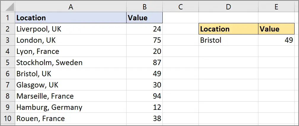
The following formula has been used in cell E3. The ampersand (&) has been used to concatenate the location in cell D3 with the asterisk wildcard. So this VLOOKUP will find the first value that begins with the text in D3.
Sometimes you do not know, or in this case do not need to know the full name of what you are looking for, and a partial match in itself is unique.
=VLOOKUP(D3&"*",$A$2:$B$10,2,FALSE)

Wildcard Characters with COUNTIF and SUMIF
The COUNTIF and SUMIF functions of Excel are also two of its most commonly used functions. It makes sense therefore that wildcards can be used with them.
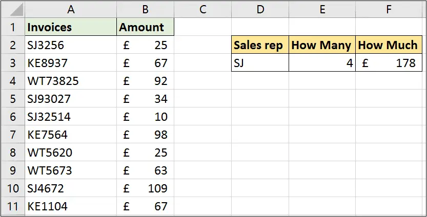
In the example below we have a list of invoices and amounts. The first two characters of each invoice determine the sales rep involved.
We do not care about the exact invoice number right now. Just as long as the first two characters match the sales rep I am reporting on, then fantastic.

This COUNTIF function was used in cell E3 to calculate the number of orders by the sales rep SJ. In similar fashion to the preceding VLOOKUP example, cell D3 and the asterisk character are joined to create the criteria.
=COUNTIF(A2:A11,D3&"*")
This SUMIF function was then used in cell F3 to total the orders for SJ, or whatever sales rep is entered into D3.
=SUMIF(A2:A11,D3&"*",B2:B11)
Not all functions can accept the direct use of wildcard characters like this. A noticeable function in this list is IF. To check for a partial match with IF in Excel, the SEARCH and ISNUMBER functions are used.
Count Cells Containing a Specific Number of Characters
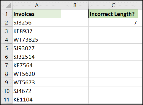
In this example, we imagine a list of invoice numbers which should all be 6 characters in length. We want to test the range of invoice numbers to check if there are any inconsistencies.
The formula below uses a COUNTIF function and the question mark wildcard. By entering 6 question marks in a string we are counting the cells containing exactly 6 characters.
The answer in cell C2 is 7 indicating that there must be 3 that do not meet that criteria. Can you see them? Well in the next example we will get Conditional Formatting to highlight them.
=COUNTIF(A2:A11,"??????")

Identify Cells with Incorrect Text Length using Conditional Formatting
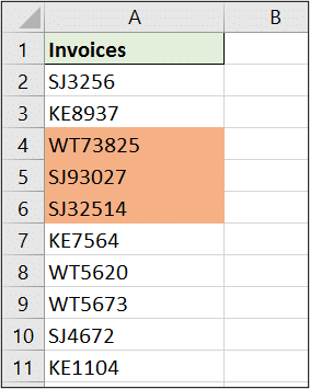
This formula can be added into a Conditional Formatting rule to identify the cells containing the incorrect text length.
The formula below has been used. It is slightly different to the COUNTIF in the previous example.
=COUNTIF(A2,"<>??????")
Because it is part of a Conditional Formatting rule, it only references the single cell (A2). This is the first cell of the range. The formatting is applied to the entire range of cells, but in the formula you reference just a single cell.
If you are not familiar with the “<>” symbol, that is the NOT operator. It has been included in the string with the six question marks. So this rule will format all the cells that do not have 6 characters.

Wrap Up
Wildcard characters can be used in more functions that what I have demonstrated here. Using them with IF, FIND and SUBSTITUTE can be useful also.
If you can perform formulas on the full content of a cell that fantastic, but when you do not know the full content, wildcards do a great job of stepping up to the plate.


Very useful information, Alan. Many thanks for sharing.