VLOOKUP is an awesome Excel function. One of its limitations is that it can only return the first match from a list. In this tutorial, we will see how to use VLOOKUP for the last match in Excel.
VLOOKUP is typically used to look for a unique value. But what about when the value you are looking for appears multiple times in the list, and you want to return the last match.
Sure we could sort the list so that the last match would become the first, but this is not always an option.
This tutorial uses VLOOKUP for the last match. The formula used can be adapted to find the 2nd or 3rd match, if required.
VLOOKUP for Last Match – Watch the Video
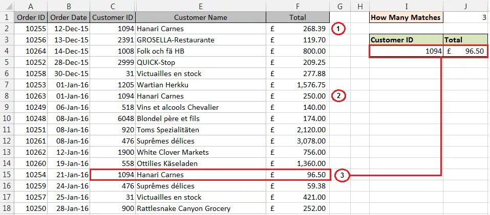
In order to create a VLOOKUP to return the last match in the list, we will need to know how many matches there are in total.
The following formula has been entered in cell J1 to return how many times the customer ID occurs in the list.
=COUNTIF(C:C,$I$4)
Create a Helper Column for the Lookup Value
Next we need to create a column of unique values which can then be used by the VLOOKUP function.
The values in this column are made by joining the customer ID and that instance of the ID. The image below shows column D as the helper column. You can see the two instances of customer Hanari Carnes which has the ID 1094. A number 1 and 2 has been attached to the end of the ID to make it unique.
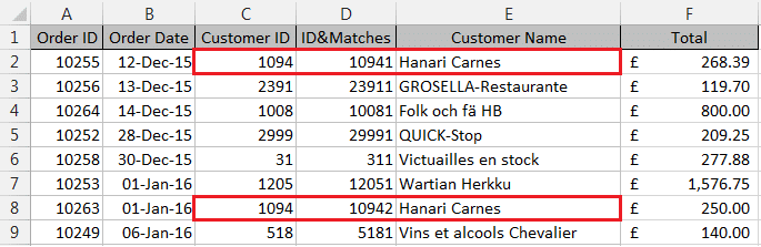
The following formula has been entered into column D. The position of the dollar signs is important for this formula to work.
=C2&COUNTIF($C$2:$C2,C2)
The COUNTIF function is an extremely powerful and versatile function to have in your Excel arsenal. Check out these 5 alternative examples of the COUNTIF function.
This column can be hidden once the VLOOKUP is written. It is an important column, but it does not need to be visible on screen.
VLOOKUP Function for the Last Match
With the helper column now in place, we can write a VLOOKUP to look to return the last match in a list.
The VLOOKUP function below has concatenated the contents of cell I4 (the customer ID) and J1 (the number of occurrences in the list of that customer ID) together to form the lookup value.
The table array is columns D:F to ensure that the leftmost column of the array is the helper column that we created.
=VLOOKUP(I4&J1,D:F,3,FALSE)
Want more information on VLOOKUP? Check out the ultimate guide to VLOOKUP.


Leave a Reply