SEQUENCE Function in Excel

In this tutorial, we will introduce you to the fabulous SEQUENCE function in Excel along with two ‘real world’ examples of its use.

The SEQUENCE function is a dynamic array function and is only available in Excel 365, Excel 2021 and in Excel Online.

When you first see the SEQUENCE function, it is maybe not that clear how it will come in useful. So, two examples will be provided toward the end of this tutorial, and in the following video, to see some practical uses.

You can download the Excel workbook used in this tutorial to follow along.

SEQUENCE Function in Excel

The SEQUENCE function produces a sequence or series of numbers. It accepts four arguments, although only the first one (rows) is mandatory.

=SEQUENCE(rows, [columns], [start], [step])

• Rows: The number of rows to return.
• Columns: The number of columns to return.
• Start: The first number in the sequence.
• Step: The amount to increment each subsequent value in the sequence.

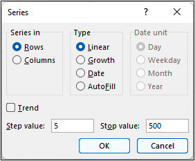
You may recognise these arguments from the Series window of Excel that you can access by clicking Home > Fill > Series. SEQUENCE is the formula equivalent of how we can generate a series of numbers by dragging the fill handle, or by using this window.

Generating a Series of Numbers Down Rows

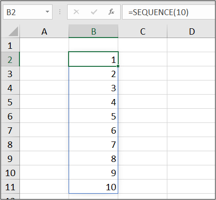
For a quick example of using SEQUENCE in Excel, the following formula generates a simple number series from 1 to 10 down rows. Only the rows arguments of SEQUENCE was used. The start value of 1 and step value of 1 were assumed, as they were not specified.

=SEQUENCE(10)

Using the Columns Argument

In this example, we include the columns argument of the SEQUENCE function in Excel. This produces a sequence down 10 rows and across 2 columns.

=SEQUENCE(10,2)

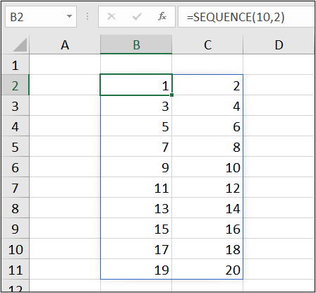
Notice, that the order of the sequence goes across columns before going down the rows. We will look at how to change to order of these two-dimensional sequences soon.

Using All the Arguments

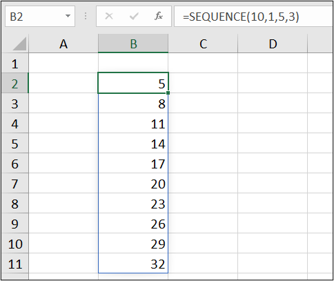
Let’s now add the start and step arguments to our formula. The following example, returns an array of values 10 rows in height and 1 column wide. It starts from number 5 and steps every 3.

=SEQUENCE(10,1,5,3)

Reversing the Sequence

It is possible to enter a negative value for the step argument of the SEQUENCE function. By doing so, we can reverse the order of the sequence.

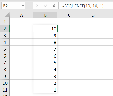
The following formula generates a series of numbers from 10 down to 1. Notice that the columns argument was skipped this time.

=SEQUENCE(10,,10,-1)

Change the Rows/Columns Order

We saw in a previous example, that when given a two-dimensional array, the SEQUENCE function returns a series that orders across columns before down the rows.

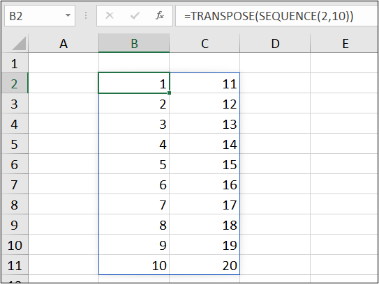
This order can be changed by wrapping the TRANSPOSE function around SEQUENCE. The number of rows and columns have also been reversed.

So, SEQUENCE is told to return and array of 2 rows and 10 columns, and then this is transposed. Pretty cool!

=TRANSPOSE(SEQUENCE(2,10))

Example 1: Return the Last N Days Sales

Let’s now look at the first example of using the SEQUENCE function in a practical scenario.

We have the following table of sales data named tblSales. It contains thousands of rows with the date of the sale recorded in the [Date] column and its value in the [Sales] column.

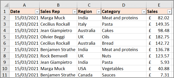
We will create a report with the total sales for each of the last N days. The number of days will be specified by a cell value.

This SEQUENCE formula is entered into cell B6 and can be seen in the following image. It uses the date in cell B3 as the start value, returns the number of rows specified in cell C3 and has a step value of -1.

=SEQUENCE(C3,,B3,-1)

And the following SUMIFS function has been used in cell C6. It references all the returned dates with the spill reference B6#.

=SUMIFS(tblSales[Sales],tblSales[Date],B6#)

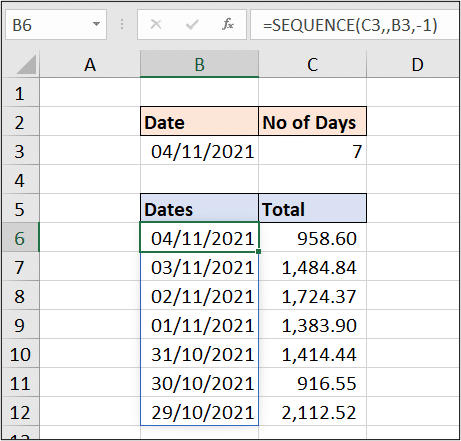
This returns the 7 days leading up to and including the date in cell B3. Awesome!!

Example 2: Sum the Top N Values

For our second SEQUENCE function example, we will sum the top N values from the [tblSales] table.

In the following formula, the SEQUENCE function is nested within the LARGE function to return the sequence of {1,2,3}. The sequence is specified by the value in cell E3. LARGE then returns the largest three values to be summed.

=SUM(LARGE(tblSales[Sales],SEQUENCE(E3)))

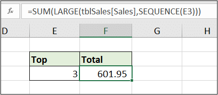
This formula is dynamic and the value in cell E3 can be changed to sum any top N values you may want.

This is easier than using the SUMPRODUCT function or some other array formula, as we have done in the past.

So, the SEQUENCE function in Excel is absolutely fantastic. Go and experiment with what else it can do. It complements the array engine of Excel very nicely.