A common requirement in Excel is the need to separate text into different cells. The reasons for this are numerous, but typically it is because the way the data was imported or received is not sufficient for your analytical needs.
This tutorial looks at four techniques for separating text.
- Using Text to Columns to separate text
- Extract name from an email address
- Extract text between two characters
- Separating a number from text
Using Text to Columns to Separate Text
Excel has a built-in feature for separating text into different cells and it is known as Text to Columns. It is very good and easy to use.
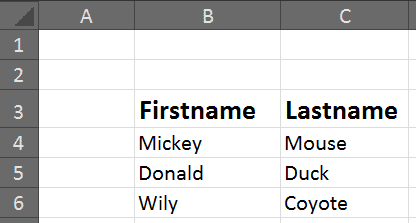
Let’s have a look at it being used to separate names into different cells.
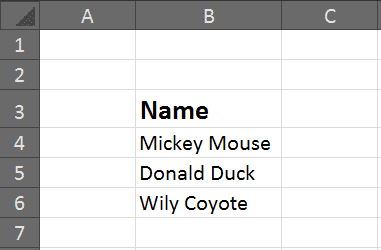
- You should first ensure that you have an empty column to the right of the range containing the data for separation (like in the image above). If not, the Text to Columns feature will warn you that it will overwrite the contents of this column. Alternatively, you can also specify a destination cell in the final step of the Text to Columns wizard.

- Select the range containing the data you want to separate.
- Click the Data tab on the Ribbon and then Text to Columns.
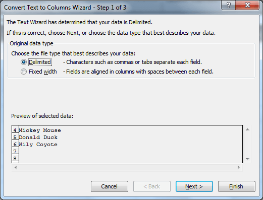
- The Convert Text to Columns Wizard appears and asks how to separate the text. The feature automatically detects that the data is delimited. If not, the fixed width option enables you to specify where the separation should occur.
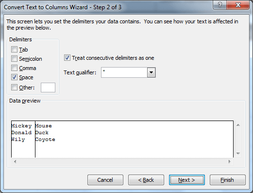
- Step 2 asks what delimiter character is being used to separate the text. In this example the delimiter is a space. Check the space box and ensure others are unchecked.
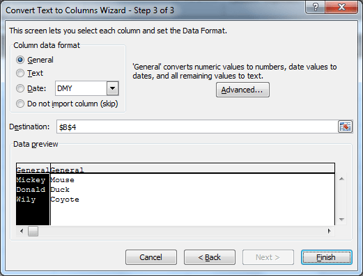
- Step 3 provides formatting options for the columns. This is not necessary in this example. Click Finish.
- The text is separated. Enter appropriate headings for the columns.
Watch the Video
Extract Name from an Email Address
Another common requirement is the need to extract a name from an email address. The image below shows names in column C that have been extracted from the email addresses in column B.
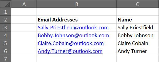
The following formula was written in cell C3 and copied down to achieve this.

- The LEFT function is used to extract text from the beginning of another piece of text. It has been used in this formula to extract al the text to the left of the ‘@’ symbol.
- The FIND function is used to return the position of one piece of text inside another. In this formula, it has been used to find the ‘@’ symbol for the LEFT function.
- The SUBSTITUTE function is then used to replace the ‘.’ In the email address with a space.
Watch the Video
Extract Text between Two Characters
To extract text between two characters will be more complex. In the example below, the text in column C has been extracted from between the two ‘/’ in column B.
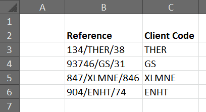
The formula below has been used to achieve this.

- The LEFT function has been used to extract text from the beginning of a piece of text.
- In the first part of the LEFT function, a MID function is used to return all the text after the first ‘/’. FIND has been used to locate the ‘/’ and LEN used to return all the remaining characters.
- In the second part of the LEFT function, the same MID function has been used to return everything after the first ‘/’. This time though it is combined with another FIND function to get the position of the other ‘/’ in the extracted text. 1 is then subtracted to return the number of characters LEFT needs to extract.
Not a straightforward formula, but hopefully that makes some sense.
Watch the Video
Separate a Number from Text
Separating a number from text will be more difficult. It can be done using a formula but it would require a chunky array formula. Therefore I opted for a VBA solution.
The image below shows the numbers in column C that have been extracted from the text in column B using this macro.
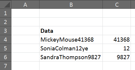
The VBA code below can be used to separate a number from text in a cell. Comments have been added to the code for explanation.
Sub ExtractNumber()
Dim i As Integer 'To count throught the characters in a cell
Dim rng As Range 'Range object to loop through all the cells in the selected range
Dim TestChar As String 'The characte being tested
Dim IsNumber As Boolean 'Used as a way of exiting the loop when a number, or text has been found
Dim StartChar As Integer 'Stores the position of the first number in the text
Dim LastChar As Integer 'Stores the position of the last number in the text
Dim NumChars As Integer 'Stores how many numbers there are for extraction
'Loop for each cell in user selection
For Each rng In Selection
    IsNumber = False
    i = 1
    'Loop to identify position of first number in the text
    Do While IsNumber = False And i <= Len(rng)
    TestChar = Mid(rng, i, 1)
    If IsNumeric(TestChar) = True Then
        StartChar = i
        IsNumber = True
    End If
    i = i + 1
    Loop
    IsNumber = False
    'Loop to identify the last number in the text
    Do While IsNumber = False And i <= Len(rng)
    TestChar = Mid(rng, i, 1)
    If IsNumeric(TestChar) = False Or i = Len(rng) Then
        If i = Len(rng) Then
            LastChar = i
        Else
            LastChar = i - 1
        End If
        IsNumber = True
    End If
    i = i + 1
    Loop
    NumChars = LastChar - StartChar + 1
    rng.Offset(0, 1).Value = Mid(rng, StartChar, NumChars)
Next rng
End Sub
Subscribe to the Excel VBA course to learn more about these techniques and much more.


Hi,
Nice to see to video and your webpage. I tried your code, it works well.
If I have a text like ” 99 45.2 87.2369 ” in a cell, how to separate the above string in to three numbers. That is 99, 45.2, 87.2369
Any help.
Thanks.
Regards,
KMOthpur
Well, the string has spaces in between…..in my above comment…..
Hey, a great piece of code which I have used, however I found a small issue with the last for loop and had to change it to :
If i = Len(rng) Then
LastChar = i
Else
LastChar = i – 1
it then removed the letters from the end
Great code..
I have one slight variation. What if the string value is MCPT9-30390 and I need to return 30390.. The code returns 9 which is the number after “T”. How best to modify the code to return 30390 if only one cell in the selection contains that string ?
We can use the – as the delimiter. Assuming the value is in cell A1 you could use =MID(A1,FIND(“-“,A1)+2,5). This will work in the example you gave. You may need more if the values are more random.
Hello,
I am trying to do something similar. I am trying to extract two numbers relative to the character “x” in a given string. I want to extract the number just before “x” into one cell, and the number just after “x” into another cell.
Example:
String:
24″ X 37.5′ cut to length with notches[etc.,etc.]
Output:
field1.Value = 24
field2.Value = 37.5
Any ideas?
Hi John, in the formulas below I have assumed that there will always be double inverted commas at the end of the values.
To extract the number before the X I used;
=VALUE(LEFT(A1,FIND(“”””,A1)-1))
And to extract the one after the X I used;
=MID(A1,FIND(“X”,A1)+2,FIND(“*”,SUBSTITUTE(A1,””””,”*”,2))-FIND(“X”,A1)-2)
These formulas assume that the number is in cell A1.
I hope this helps.
Alan
Well, that’s a formula, but how would you modify -Sub ExtractNumber ()- to incorporate that formula? For instance, if you had textbox within a userform called “comments” which contained the string, and you wanted to use a command button to output the two numbers (from “comments”)to textboxes “field1” and “field2” (within the same userform) respectively?
Thanks so much for your reply, by the way!
Posting this reply as a comment:
How would you modify -Sub ExtractNumber ()- to incorporate that formula? For instance, if you had textbox within a userform called “comments” which contained the string, and you wanted to use a command button to output the two numbers (from “comments”)to textboxes “field1” and “field2” (within the same userform) respectively?
hi the code helped me in my task but i have one issue my text is MEDIA SOLUTIONS (1005) and i want only 1005 when i run the above code the result is 1005) , how can remove the last bracket and get only 1005
Hi Ashwini,
Lets imagine the text MEDIA SOLUTIONS (1005) is in cell A2. You could use the formula below.
=MID(A2,FIND(“(“,A2)+1,4)
Kind regards
Alan
Sir;
I has run the cod but it is not working. My data is as fellow
persone1person2person3person4
When i run the code, it only give 1 while i am expecting that it should return 1234.
Kindly let me know that where is the issue
Yes this macro only works with contiguous numbers. It would not work for your scenario. You would need a macro to keep checking after the first extraction and to join the results together.
hi enjoyed the you tube tutorial. not a programmer but trying to use this to extract number from 7.2 degree centigrade symbol the result would be 7. even if i format cells i only get 7.0
sorry to trouble you with this.
this is personal work not commercial
best regards martin
Hi Martin,
Thank you for your comments on my YouTube video.
If the temperature is in cell A2, you could use this formula to extract the 7.
=VALUE(LEFT(A2,FIND(“.”,A2)-1))
Or the below to get the 7.2.
=VALUE(LEFT(A2,FIND(” “,A2)-1))
Hi? How do you separate a decimal number from texts e.g. a number like fghr456.321
Hi? I liked the macro code but now how do you separate a decimal number from texts e.g. a number like fghr456.321 well i expect the number to be 456.321 and not 456
Hi Solomon,
In the line of code found below;
If IsNumeric(TestChar) = False Or i = Len(rng) Then
Try adapting it to add in the part highlighted in bold. I think this will work.
If IsNumeric(TestChar) = False Or TestChar = “.” Or i = Len(rng) Then
I hope this helps.
Alan