Non-Adjacent Columns with FILTER Function

This tutorial will return non-adjacent columns with the FILTER function. Dynamic array functions such as FILTER and SORT can only return consecutive columns natively. However, there are various methods to specify the columns to return from the array. Functions such as CHOOSECOLS, CHOOSE and INDEX are wonderful for this task.

You can download the Excel workbook to follow along

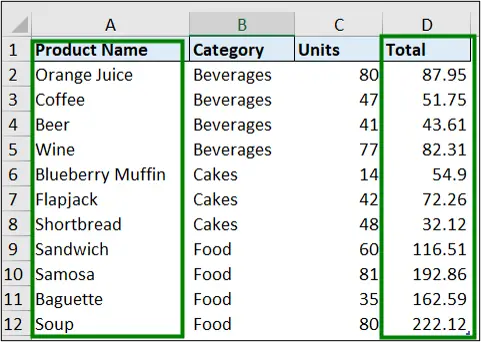
The table below is named tblSales. We will use a FILTER function to return the results of the [Product Name] and [Total] columns only.

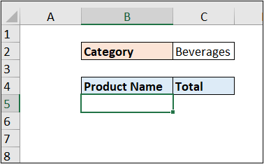
Below is a prepared report to return the product name and total columns for the product category stated in cell C2. Currently, beverages.

There are two key approaches to doing this. We can use absolute references to the columns by name e.g., tblSales[Product Name], or reference them using their column index numbers.

1. Absolute: The CHOOSE function can be used to reference the columns in an absolute manner. This is especially useful when your data is formatted as a table, like it is in this example as tblSales.
2. Dynamic: The CHOOSECOLS or INDEX functions are great for relative referencing of the columns using their index numbers. This can be made more dynamic with the help of functions such as SEQUENCE, MATCH and COLUMNS.

CHOOSECOLS offers the easiest way to return non-adjacent columns from an array, but it is only available in Excel 365 and Excel Online. If you don’t have it, consider using the INDEX function. It is just as capable.

Let’s begin with CHOOSECOLS.

Non-Adjacent Columns with CHOOSECOLS

In cell B5, we will enter the FILTER function. Its syntax is shown below.

=FILTER(array, include, [if_empty])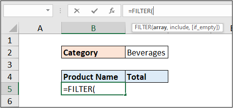

• array: The array argument is the columns in the tblSales table we want to return. These are the [Product Name] and [Total] columns, which are columns one and four respectively. The CHOOSECOLS function will be used here. CHOOSECOLS is built to return specific columns from an array or range. The columns to return are provided as numbers in separate arguments.
• include: The include argument is our filter criteria. In this case, we want to return the products from the product category stated in cell C2 only, currently beverages. So, our filter criteria will be when the [Category] column equals the value in the cell C2 e.g., tblSales[Category]=C2.
• [if_empty]: This argument is an optional argument and will be ignored in this formula. It is used to suppress the CALC! error, which is returned if the FILTER function has no results to return, and provide an alternate result.

Therefore, the formula in cell B5 is written as

=FILTER(CHOOSECOLS(tblSales,1,4),tblSales[Category]=C2)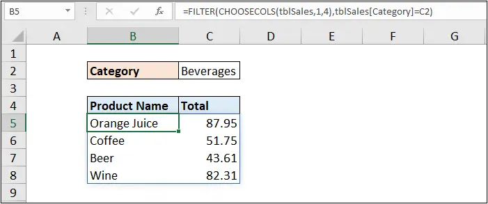

We have successfully returned the [Product Name] and [Total] Columns only.

Using CHOOSE for Absolute Column References

We can also return non-adjacent columns from an array with absolute references using the CHOOSE function in Excel.

To do this, we will use the CHOOSE function in the array argument of the FILTER function. The syntax of the CHOOSE function is as follows.

=CHOOSE(index_num, value1, [value2],...)

• index_num: The index number specifies the value argument that is selected. In this scenario, for our index_number, we used the array of constants: {1,2}. This means to return value1 and then value2 in that order.
• value1, [value2], …: The list of values or actions that CHOOSE will return. CHOOSE will return the value that corresponds to the given index_num. Value1 is only required value. In this example, we used the column names we want to return from the tblSales table rather than using the column numbers 1 and 4 used in the previous example.

The following uses the CHOOSE function to return non-adjacent columns with dynamic array formulas.

=FILTER(
CHOOSE({1,2},tblSales[Product Name],tblSales[Total]),
tblSales[Category]=C2)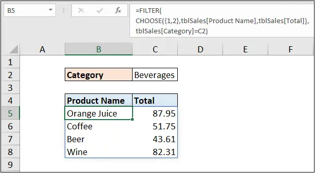

Using SEQUENCE to Prevent Column Index Numbers

The SEQUENCE function is used to generate a list of sequential numbers in an array form. The dimension returned is dependent on how many rows and columns we specify.

SEQUENCE can be used to return a list of column numbers, saving us the task of manually entering the column index numbers. This could be as simple as the sequence {1, 2} used in the previous example, or another sequence such as {2, 4, 6, 8}.

The SEQUENCE function has been used to replace the array of constants of {1, 2} used previously. The following describes how SEQUENCE has been used.

• rows: The rows argument returns the number of rows specified. In our current example, we don’t need this argument as we want to return columns only.
• [columns]: The column argument is optional, however, the rows or columns argument must be used, and as we are ignoring rows, we must provide this. In this example, we want to return two columns: [Product Name] and [Total].
• [start]: This argument was ignored. It is the number to start the sequence from, and if ignored 1 is used.
• [step]: This argument was also ignored. It is the number to step in the sequence, and if ignored, a step of 1 is used.

The following formula uses the SEQUENCE function with CHOOSE to return non-adjacent columns with dynamic array formulas.

=FILTER(
CHOOSE(SEQUENCE(,2),tblSales[Product Name],tblSales[Total]),
tblSales[Category]=C2)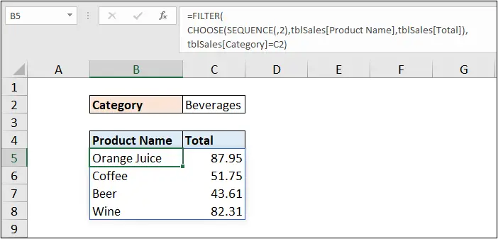

Return Non-Adjacent Columns Dynamically with CHOOSECOLS & MATCH

In this example, we want to dynamically reference the columns in our tblSales table. To do this, we have used CHOOSECOLS with the MATCH function to lookup the headers required (these are entered in cells on the sheet) in the tblSales table, and return their column index numbers.

This prevents us from needing to enter the column numbers manually, and also means that if a cell value is changed, the new column header is returned.

Let’s take a look at how the MATCH function will be used.

• lookup_value: The lookup_value is the value we want to return in the lookup_array. In our formula, the lookup values are the headers entered in range B4:C4 on the report sheet. This means that the header names in range B4:C4 of the report sheet must match the names of the headers in tblSales.
• lookup_array: The lookup_array is where you are looking for the lookup_value. In our formula, we have referenced the header row of the table: tblSales[#Headers].
• [match_type]: The [match_type] argument specifies whether we want to return an exact match or other options. In this example, we used 0 as we want an exact match.

The following is how the CHOOSECOLS and MATCH functions have been used with the FILTER function in our formula.

=FILTER(
CHOOSECOLS(tblSales,MATCH(B4:C4,tblSales[#Headers],0)),
tblSales[Category]=C2)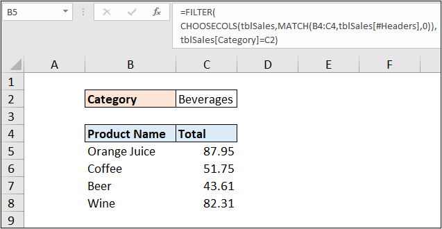

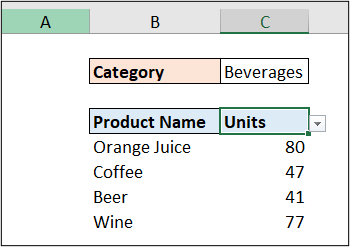
The formula gives us the same result as previous ones. But this time, using a drop-down list in cell C4, we can change the [Total] column to [Units] and it will return the total units instead. This demonstrates the dynamic nature of this formula.

INDEX & MATCH to Dynamic Reference Non-Adjacent Columns

CHOOSECOLS is a recent function in Excel and not everyone has it. In this section, we demonstrate how to use the INDEX function in the formula instead of CHOOSECOLS. The INDEX function is super versatile.

Let’s take a look at how the INDEX function has been used.

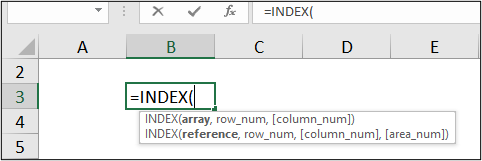
• array: The array argument is the data that you are returning from and can be a range, table or an array. In our formula, the array argument is the tblSales table.
• row_num: The row_num argument is the row position in the array for the value that you want to return. For this formula, we needed to request all rows of the table, so the ROWS function was used within SEQUENCE. The ROWS function tells SEQUENCE how many rows are in a table and SEQUENCE generates the array of row numbers from 1 to the total number of rows.
• [column_num]: The [column_num] argument the column position in the array for the value that you want to return. In this formula, the MATCH function is used here to lookup the column headers and return the array of column index numbers.

The following is how INDEX & MATCH have been used with FILTER to return non-adjacent columns with dynamic array formulas;

=FILTER(
INDEX(tblSales,SEQUENCE(ROWS(tblSales)),
MATCH(B4:C4,tblSales[#Headers],0)),
tblSales[Category]=C2)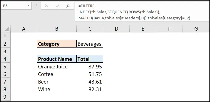

These are fantastic ways that you can return non-adjacent columns with dynamic array formulas. There is no right way, just the one that fits your needs, and version of Excel.

I hope you found this article helpful?

Please leave us a comment below.