The N function returns a number when given a value. This tutorial breaks down the N function in Excel and then shows two real-world examples of using it with the SUMPRODUCT function.
You can download the Excel workbook to follow along.
The N Function only has one argument; the value.

- value: The value argument converts a non-number value to a number. This means that it returns a number when given a value. It returns dates to serial numbers, TRUE and FALSE values to 1 and 0, respectively, and any other text value to zero (0).
Let’s see the N function in action;
=N(A2)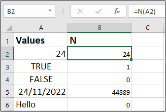
The image above shows;
The text value “Hello” returned as 0.
The date value “24/11/2022” returned as the serial number 44889.
The TRUE and FALSE values returned as 1 and 0, respectively.
That’s exactly what the N function does. The question is, why would we use the N function in our Excel formula? Let’s see some practical examples:
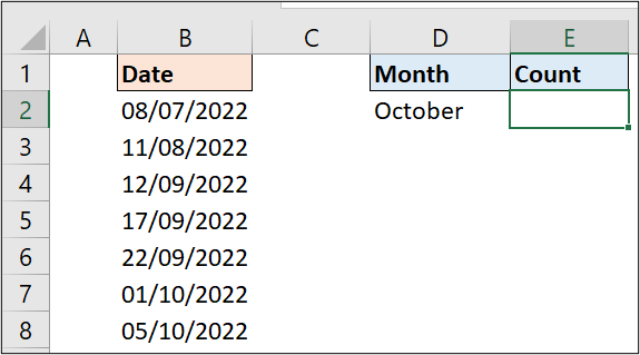
In column B of the following image, we have a list of dates. And we want to use the SUMPRODUCT function to return the number of occurrences of a specific month in cell E2.
SUMPRODUCT Function
The SUMPRODUCT function multiplies the values from a list of corresponding ranges or arrays, and then returns the sum of those values.
=SUMPRODUCT(array1,[array2],[array3],...)
- array1: The array1 is the first range or array whose values you want to multiply and then sum. In this example, this is the only array used, and it is the logical expression to return TRUE if the month of the dates in range B2:B8 is equal to October. The results are summed to produce the number of occurrences in the October month.
- [array2], [array3], …: The arrays in square brackets are optional arguments. These are ignored in this example because we only require the single test on the dates.
The result of the SUMPRODUCT function gave zero (0) despite the two October dates in the list.
=SUMPRODUCT(MONTH(B2:B8)=MONTH(D2))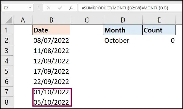
Note: In cell D2, the value (October) is a date formatted as a month name. Use the custom date format “mmmm” to achieve this.
N Function to Coerce TRUE and FALSE Values into 1 and 0
To dive deeper and investigate the problem with this formula, select the expression in the SUMPRODUCT function in our formula bar, as shown below;
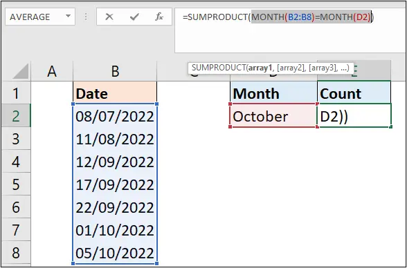
Go to the Formulas tab, and click Calculate Now in the Calculation group. We can also use the keyboard shortcut F9.

The SUMPRODUCT shows an array of TRUE and FALSE results. The SUMPRODUCT function can’t sum those values, and therefore returns zero. They must be converted into ones (1) and zeros (0) before being summed.
=SUMPRODUCT({FALSE;FALSE;FALSE;FALSE;FALSE;TRUE;TRUE})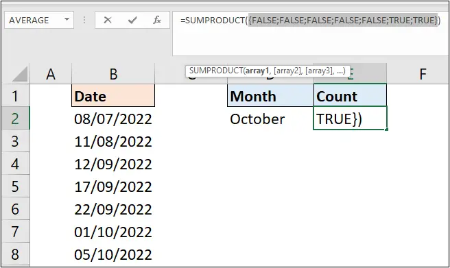
In this case, the N function can help convert the TRUE and FALSE values to ones (1) and zeros (0).
To achieve this, we wrapped the N function around that logical expression and it returned the value 2 in cell E2. This is the number of times the month of October occurred in the column of dates.
=SUMPRODUCT(N(MONTH(B2:B8)=MONTH(D2)))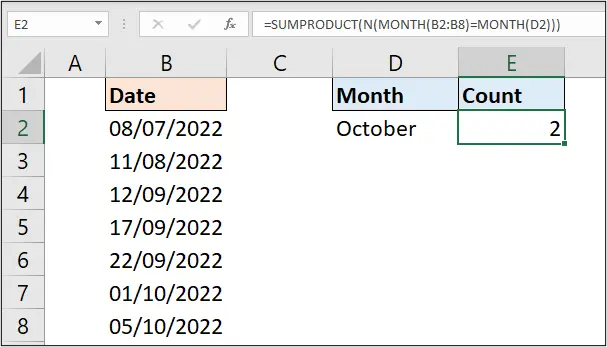
To demonstrate that the expression currently in the SUMPRODUCT function has been converted into ones (1) and zeros (0), we select the expression, go to the Calculation group in the Formulas tab and click on the Calculate Now button.
Here, we can see the values have been returned as 1s and 0s. These values can then be summed.
=SUMPRODUCT({0;0;0;0;0;1;1})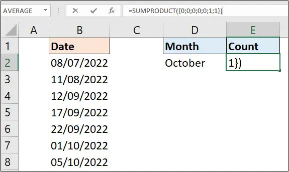
Double Negative (–) Alternative to the N Function
Some people use a double negative (–), also known as a double unary, instead of the N function to convert TRUE and FALSE values to 1 and 0.
=SUMPRODUCT(--(MONTH(B2:B8)=MONTH(D2)))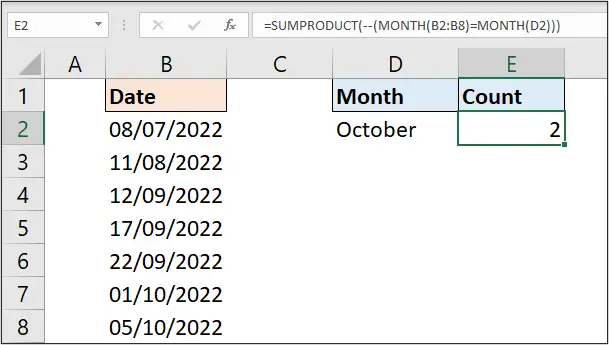
Add Comments in Excel Formulas with N Function
The most common use of the N function is to add comments to a formula. The N function can be used to display text in our formulas. Since the N function sees text values as zeros (0), when used to display text, it will not affect the result of that formula (assuming the formula returns a numeric value).
Let’s see the example below:
=SUMPRODUCT(--(MONTH(B2:B8)=MONTH(D2))+N("The month cell contains date that is formatted as a month"))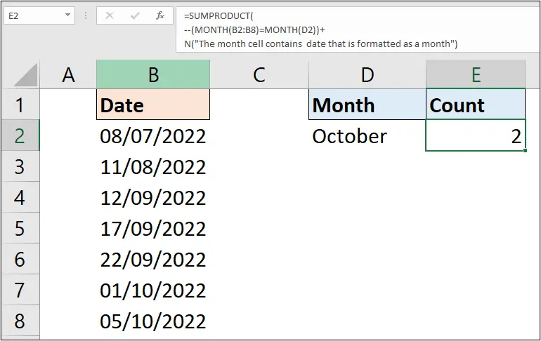
In this formula, we have put the information that says, “The month cell contains a date that is formatted as a month“. This is useful information for anywhere looking at this Excel formula. It helps explain how the expression was used to return the number of times the month occurred in the column of dates.
This is how to use the Excel N function to provide comments and documentation within a formula as an alternative to inserting a comment in a cell. Also, its use to convert an array of TRUE and FALSE values to 1 and 0 respectively.
Have you used the N function before for one of these scenarios?
Please let us know in the comments below.





Leave a Reply