Moving Average in Excel

This tutorial will look at how to calculate moving average in Excel. The moving average is sometimes referred to as the rolling average as it averages the values from a rolling, or moving, date range. In this post, our focus is on a seven-day moving average.

You can download the Excel workbook used in this tutorial to follow along.

Here in the UK, we often see an example of the graph below showing a seven-day average of 328,882.

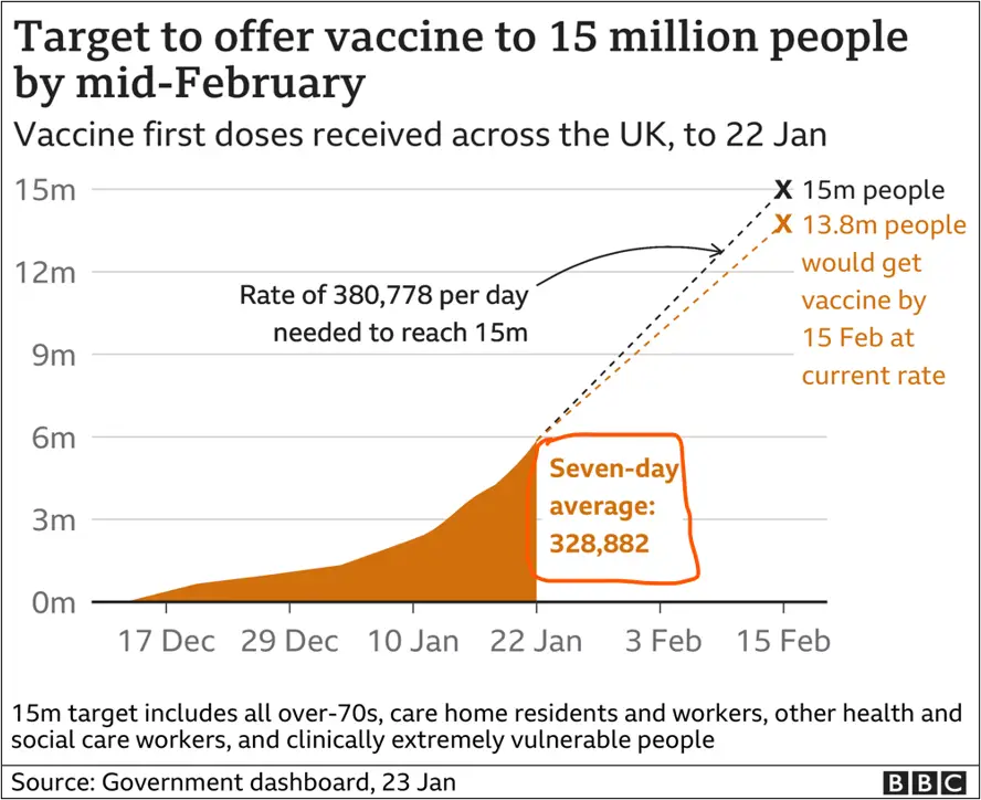
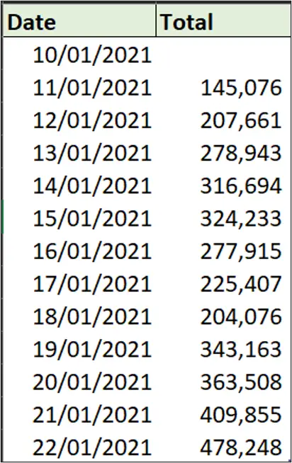
For this tutorial, we have collected the vaccination data from the 10th to the 22nd of January 2021 as used in the graph above. And we are going to calculate that seven-day average. Find the data below:

Seven Day Moving Average in Excel

The Excel formula we will use will dynamically adjust the seven day date range as new dates are added to the list, because it’s a moving average formula. This means that if we are to add the next day’s vaccine data, it will always show us the last seven day’s average.

This Excel formula can easily be adapted to whatever time frame you need for your moving average. For example a fourteen-day or six-weeks moving average.

To calculate the seven-day moving average:

In cell D3, we will enter the AVERAGE function in Excel and we need the return the last seven values. For the data to update as the number of rows increases or decreases, the data we are using is formatted as a Table named data. Hence, we will use Table references in this formula.

There are a few approaches to getting the dynamic last seven values. Possibly, the easiest approach is to use the OFFSET function. Another good function is INDEX. But it’s a little more involved. So we will use the OFFSET function for this example.

=AVERAGE(OFFSET( reference, rows, cols, [height], [width] )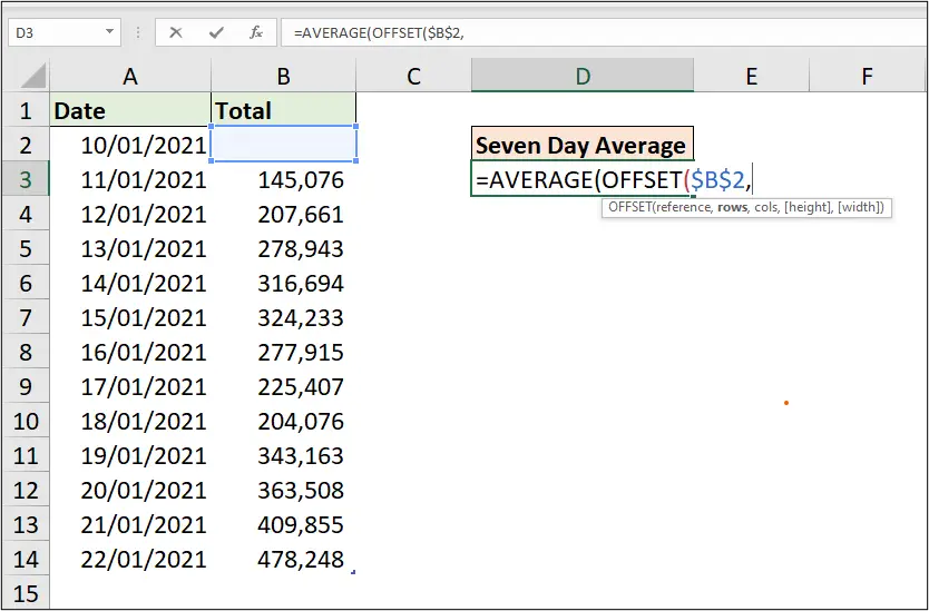

The following describes how the arguments of the OFFSET function in this Excel moving average formula have been used;

• Reference: The starting reference or cell. The start reference in this rolling average formula is $B$2 as that is the first cell in the [Total] column.
• Rows: The rows argument is where we need to find the starting value for the last seven days. So, we will use the ROWS function of Excel to fit the table (data). This will provide the number of rows that are in that table. And we minus seven from it.
• Cols: The cols argument will be ignored because we are staying in column B as indicated by our starting reference. 

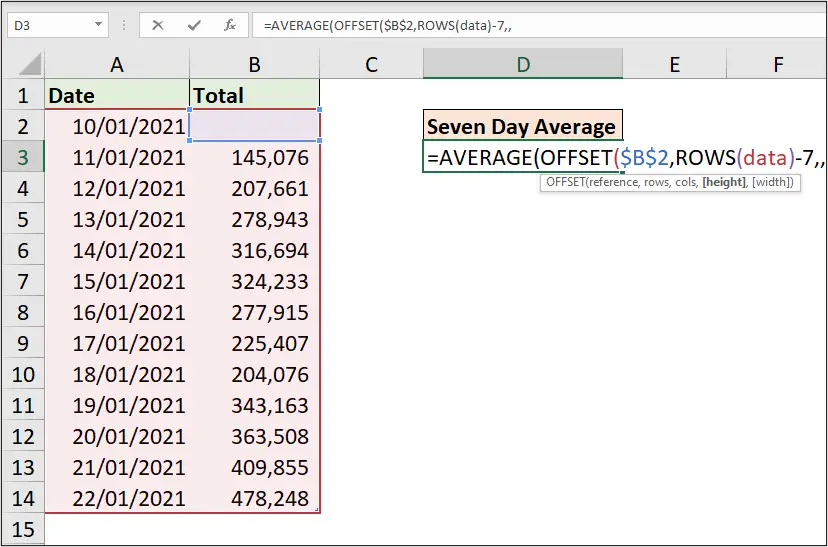
• [Height]: Seven (7) is entered as we want to return seven rows of values.
• [Width]: The width argument was omitted because the result is only one column wide.

Hence, the final Excel formula is:

=AVERAGE(OFFSET($B$2, ROWS(data)-7,,7))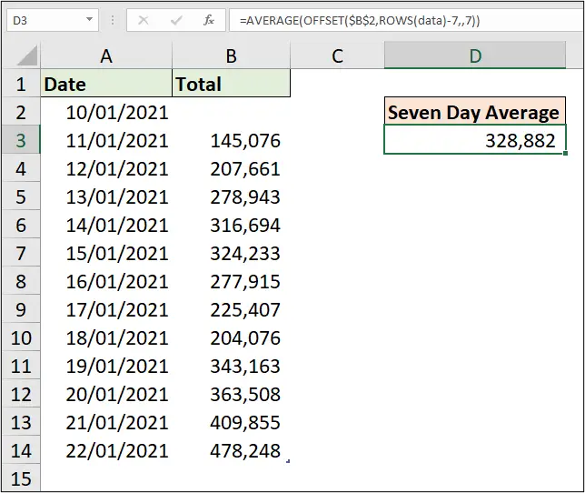

AVERAGE of the last Seven Days

Now, if we add values row 15, the value in cell D3 changes and we can verify the new value in cell D3 by using the AVERAGE function to return the average of the last seven days.

=AVERAGE(B9:B15)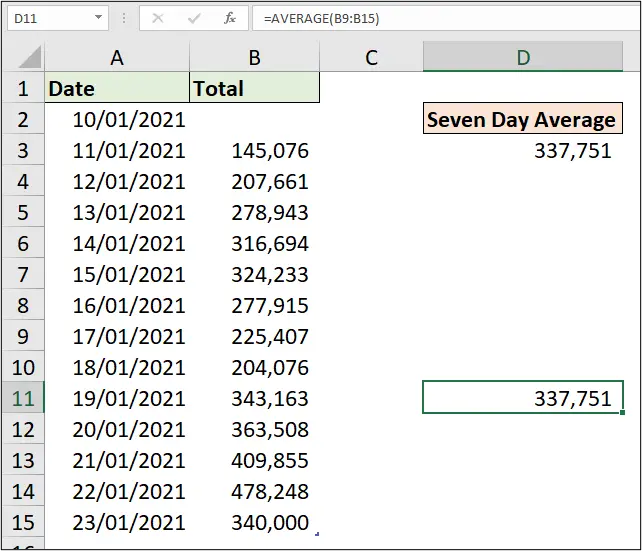

So, the moving average is a quick way to constantly return the updated average of numbers depending on the time frame you specify.

We hope you enjoyed this article? Please leave us a comment below.