Locate the Locked Cells on a Worksheet

If you wish to protect the cells on a worksheet that contain formulas you will need to lock the cells first, whilst also ensuring that the cells users should be able to change are unlocked.

It may have been a while since you worked on this worksheet and you are not sure which cells are locked and which are not. You need a fast method of locating the locked cells. Let’s use Conditional Formatting to highlight the cells that are already locked so they are easy to identify.

Highlight the Locked Cells on a Worksheet

1. Select the range of cells you want to check
2. Click the Conditional Formatting button on the Home tab and select New Rule from the list
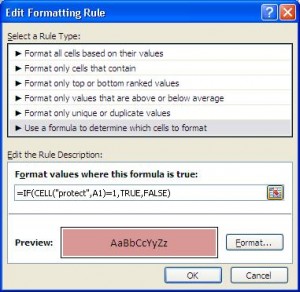
3. Select Use a formula to determine which cells to format
4. Enter =IF(CELL(“protect”,A1)=1,TRUE,FALSE) in the box provided

To identify the locked cells on a worksheet we can use the CELL function. The CELL function returns information about a cell, in this case whether it is protected. A1 represents the first cell in the selected range.

5. Click the Format button and choose the formatting you want to apply
6. Click Ok

All cells that are locked will be highlighted making them easy to identify.