When using formulas in tabular data in Excel, you will need to copy a formula down the entire column, so that each row has that same formula.
There are a few techniques to copying formulas in Excel, and this article will detail what you should be aware of, and why you would apply each specific technique.
Use the following links to jump to a specific section in the article.
- How to Copy Formulas in Excel
- How to fix a cell when copying a formula down
- Entire column formulas in Tables
- Using an array formula
Download the sample file to practise.
How to Copy Formula in Excel
To copy a formula in Excel, the easiest way is to click and drag the Fill handle that is found in the bottom right corner of a cell.
When you position your mouse cursor over the Fill handle, it changes from the standard white cross to a thinner black cross. This cursor is shown in the following image.
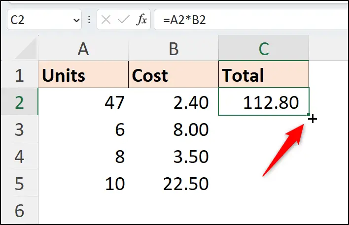
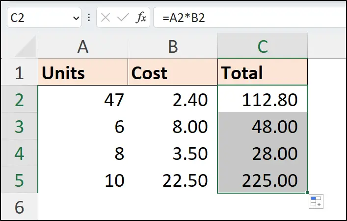
With the thinner black cross, click and drag the formula down the cells that you want to copy the formula to.
You can use this technique to copy a formula to adjacent cells in any direction – down, left, right or up). However, you cannot drag the Fill handle in a diagonal manner.
Copy Down in Excel without Formatting
In this example, we want to keep the formatting applied to all cells. However, there are options.
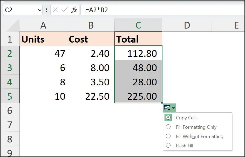
Immediately after copying the cell content, a smart tag is visible at the bottom right of the final cell that you copied to.
Click on this tag to access the Auto Fill Options. These include the option to Fill Without Formatting. By default, Excel copies everything – formula, formatting, validation, etc. However, you may want to copy only the formula.
Copy a Formula Fast to All Cells in a Column
To copy a formula down an entire column quickly, you can double click the Fill handle instead of dragging it.
This trick is fantastic. No more dragging down hundreds or thousands of cells.
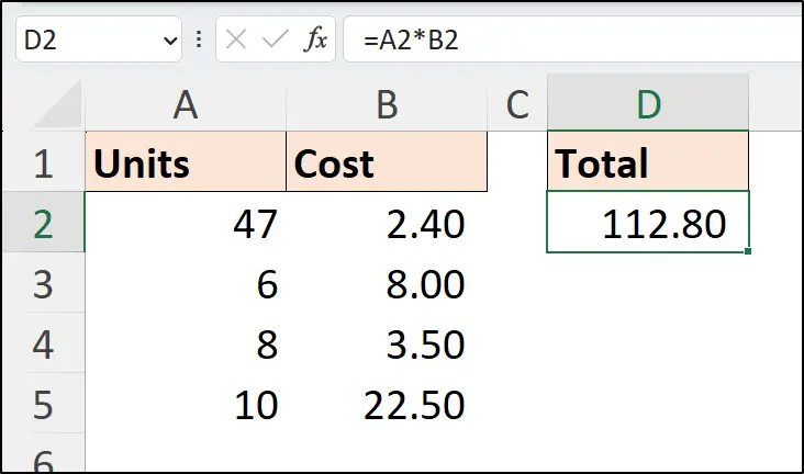
This double click trick is only possible when you have values in adjacent columns. In this example, the double click of the Fill handle will not work because the adjacent column C is empty.
Use the Fill Down Button or Keyboard Shortcut
For another method of copying formulas down a column, you can use the Fill command in Excel. This command can be accessed from a button on the Ribbon or via a keyboard shortcut.
To use the Fill command, you need to select the cells that you want to fill too. When you want to copy a formula down the whole column, this is a big limitation, and the previous techniques are faster.
To use the Fill down option,
Select the cells that you want to copy the formula to.
Click Home > Fill > Down or press Ctrl + D.
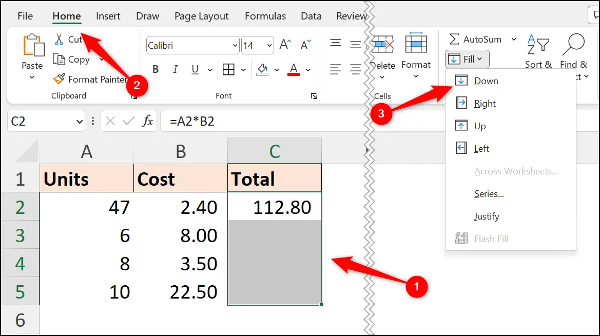
In addition to the fill down option, you can use the Fill command to copy to the right, which can also be done with the Ctrl + R keyboard shortcut.
This technique is especially useful when working with Table references in Excel formulas. We will cover using formulas with Tables later in this article.

Excel uses Relative Cell References
With all these methods to copy a formula in Excel, a relative reference has been used by default.
What does this mean?
Well, the formula reference are relative to the cell containing the formula. For example, the following formula references cell A2, which is two columns to the left of the formula, and cell B2, which is one cell to the left of the formula.
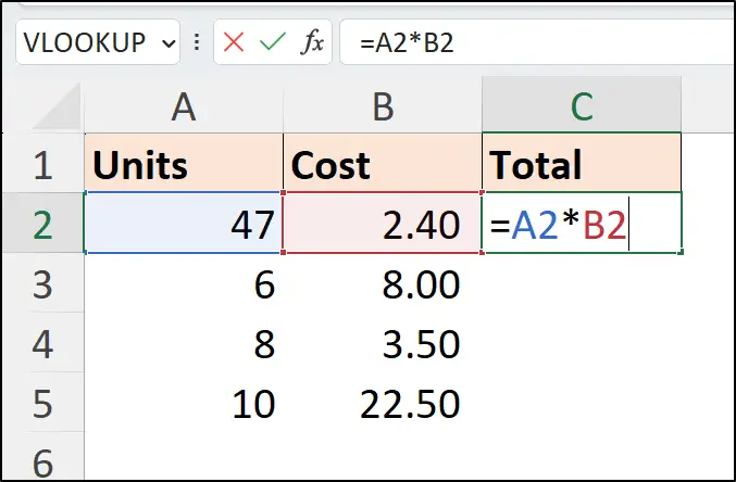
When the formula is copied down the entire column in Excel, it remains in context with the row. So, the formula in cell C4 also refers to the cells two columns to its left (A4) and one column to its left (B4).
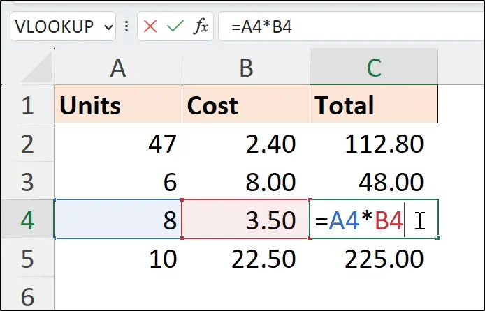
It gives the appearance that the cell reference is moving when you copy the formula, because you can see the row number of the cell address increasing. However, although the cell address is changing, it is the same reference to the relative position of the cell.
This style of referencing has been great so far, and is exactly the behaviour that we wanted when we copied the formulas.
However, sometimes you will want a cell reference to be fixed to a single cell. This is known as an absolute reference and will be covered shortly in this article.
Copying Formulas to Non Adjacent Cells
You can also copy formulas using the classic copy and paste in Excel. This is especially helpful when copying to non adjacent cells.
If you require the behaviour of a relative cell reference in your formula, ensure that when you copy and paste the formula, you select the cell(s) and use Ctrl + C or the Copy command.
Select the destination cell(s) and paste with Ctrl + V, press Enter, or use the Paste or Paste Formulas command.
In this example, after copying formulas from C3:C6, the formulas refer to cells relative to their own cell.
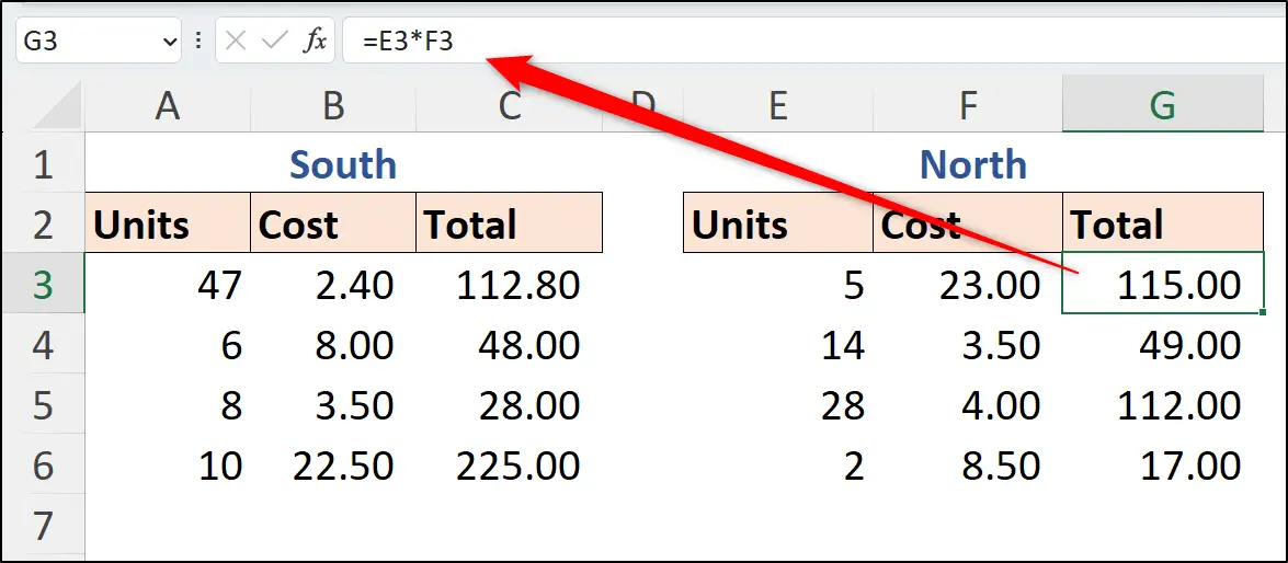
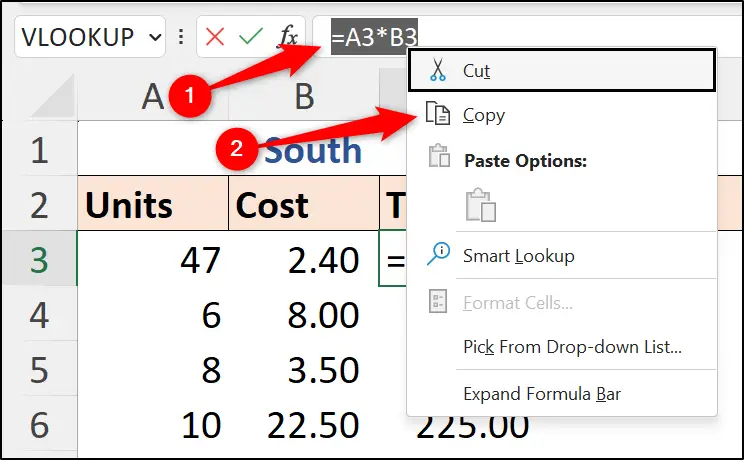
If you select the formula text in the Formula bar and copy, then the cell references do not change in the copied formula. This is a viable option if you do not want the cell references changing.
The Magic of Ctrl + Enter
By using the Ctrl + Enter keyboard shortcut you can apply a single formula to multiple non adjacent cells at once. This means you will not have to copy the formula by dragging the Fill handle or pasting formulas to multiple ranges.
Pretty cool!
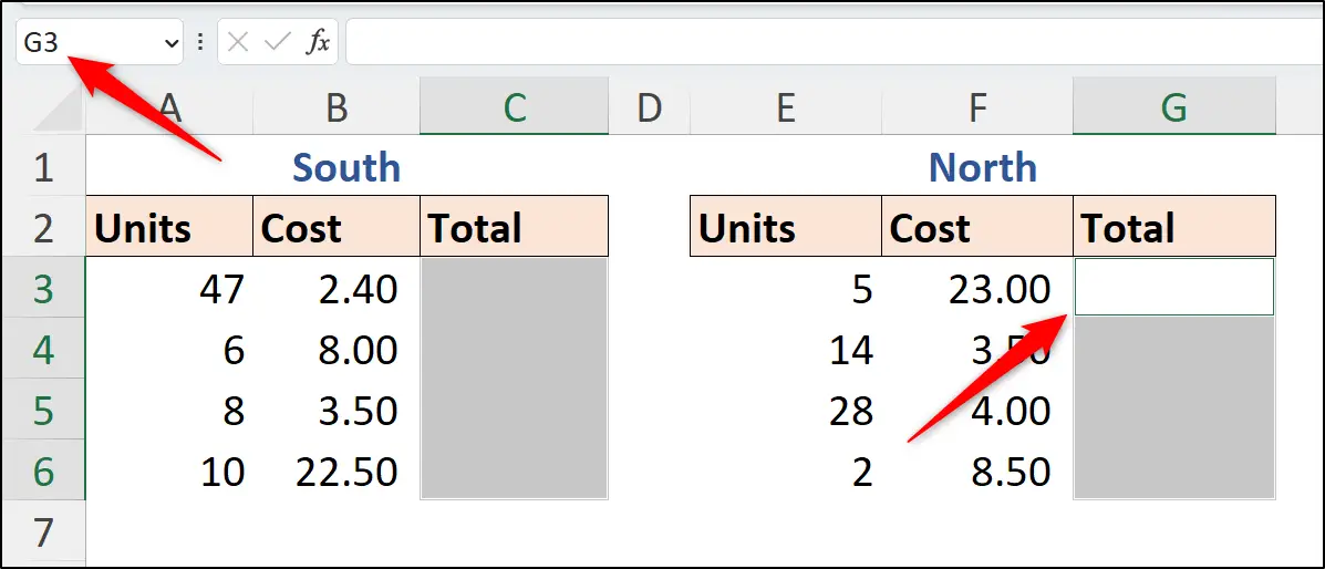
In this example, we will write the formula to the ranges C3:C6 and G3:G6 at the same time.
Select range C3:C6, press Ctrl key, and select range G3:G6, so both ranges are selected at the same time.
Notice that selecting the ranges in this order has resulted in cell G3 being the active cell. This can be identified by the white cell, and the address shown in the Name box. Because of this, the formula we write will be the one for cell G3.
Write the following formula.
=E3*F3
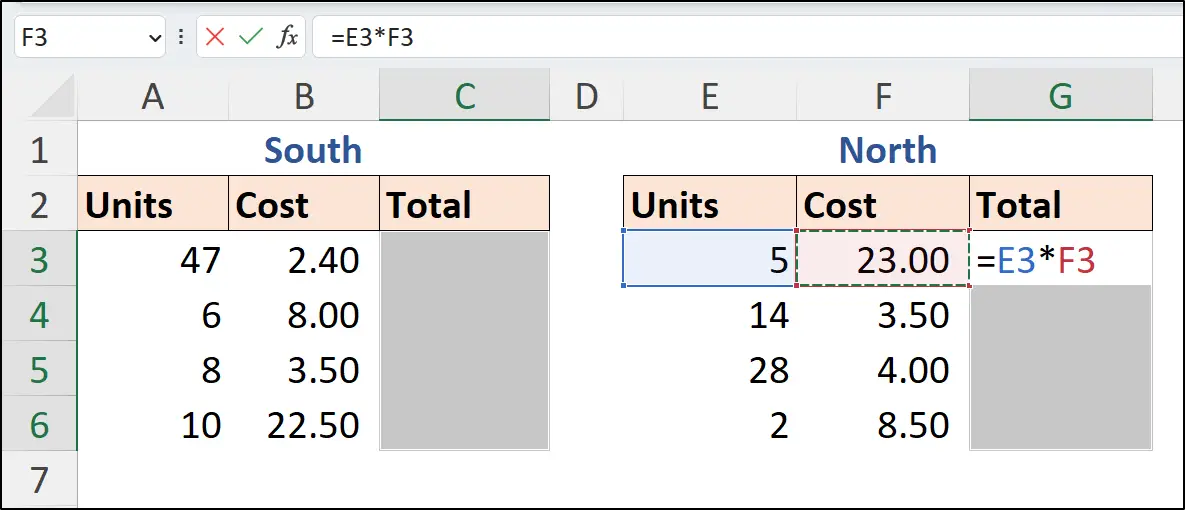
Press Ctrl + Enter.
Being able to apply a value to multiple non adjacent ranges at once is a great aspect of the Ctrl + Enter shortcut. This technique is demonstrated again in my video on how to fill blank cells with the value from the cell above.
How to Fix a Cell when Copying a Formula Down
To fix a cell and stop the address from changing when you copy a formula down, the reference needs to be made absolute.
An absolute cell reference has a dollar sign before its column letter and row number i.e., $A$2. These dollar signs fix each element of the cell address so that it does not change when the formula is copied vertically or horizontally.
Using Absolute References
All examples so far have used a relative reference in the formula. But it is now time to cover the topic of an absolute cell reference.
In this example, the formula applies the discount stated in cell D2 to the totals in column A using the following formula. However, the results in range B3:B5 are wrong.
=A2*(1-D2)
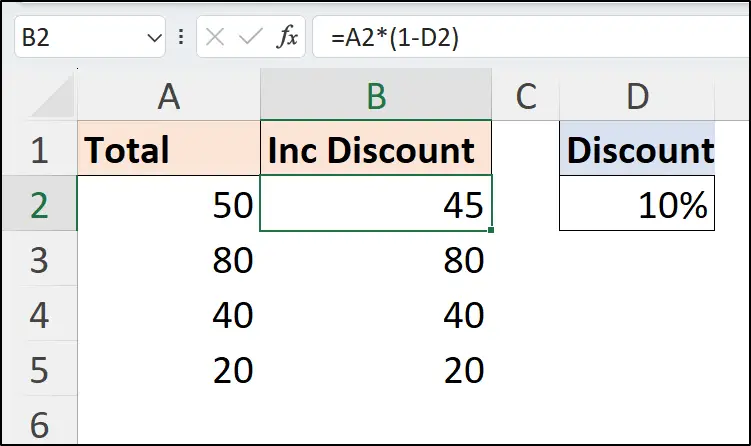
The formula has referenced cell D2 in a relative manner. Because of this, when you copy the formula down, the cell address has changed to D3, D4, and then D5.
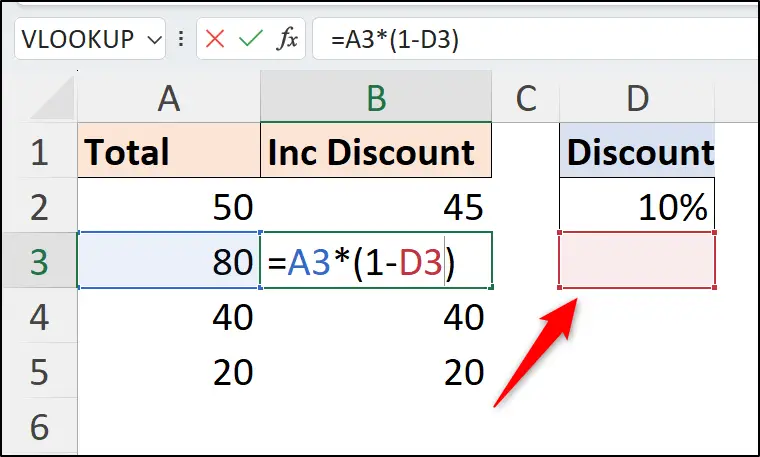
Let’s edit the original formula to stop the cell address changing when the formula is copied. To do this, dollar signs will be inserted before the column letter and row number of the address. This will fix the cell, or using its official nomenclature, make the cell address absolute.
=A2*(1-$D$2)
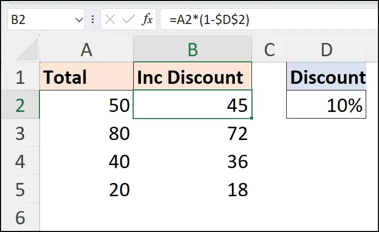
An alternative to typing the dollar signs into the formula, is to click amongst the reference in the formula and press F4 (you may need the Fn key too when using a laptop).
This shortcut will insert both dollar signs. And if you continue to press F4, it cycles through different reference styles, which we will cover next.
Mixed References in Excel
Now, in this instance, we did not require the dollar sign before both the column and row. As we are copying the formula down, it is only the row that requires the dollar.
The following formula uses a mixed reference to cell D2.
=A2*(1-D$2)
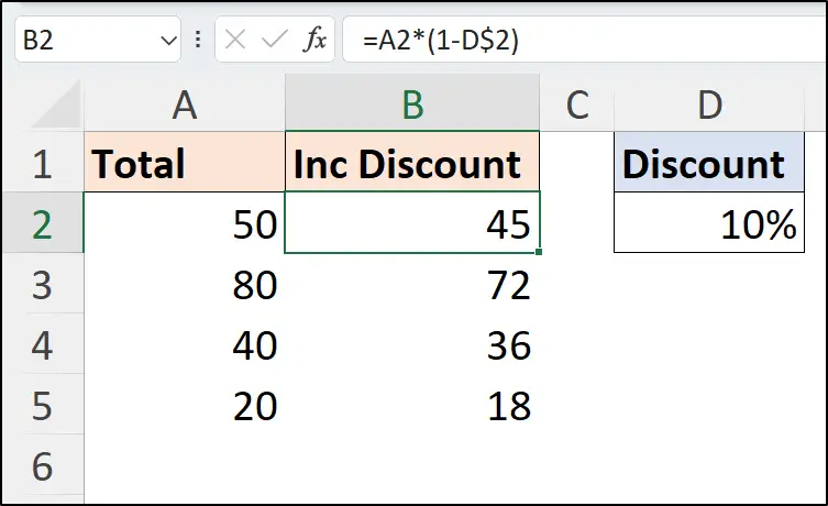
In most situations, both dollar signs would be used for an absolute reference, even though both are not necessary. It is only in more advanced situations, such as applying a Conditional Formatting rule to an entire row, when a mixed reference technique is essential.
Using a Named Range
Another method to fix specific cells is to name ranges. You can define a named range for a specific cell, a range of cells, or even a whole column or row.
To name a range;
Select the range to name.
Click in the Name box.
Type the name that you want to assign to the range (you cannot use a space, begin with a number, or use characters such as % or ! in the name).
Press Enter.
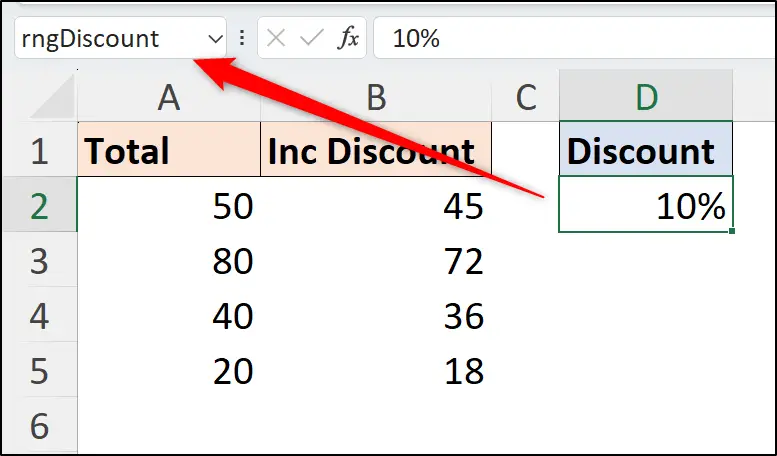
In this instance, I have prefixed the name with the letters rng to signify that it is a named range and distinguish it from other names such as Tables, named constants and named formulas. It also aids in referencing the name from within a formula.
This technique is not necessary and is just a practise that I find useful.
The named range can now be used within a formula to stop the reference changing when you copy a formula down an entire column.
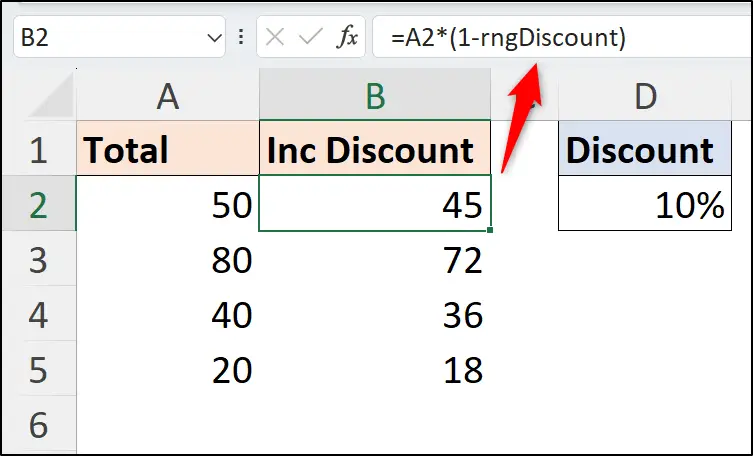
Defining names is an awesome technique in Excel that can also be used to name LAMBDA functions, constants, and name ranges using a relative address.
Entire Column Formulas in Tables
When working with tabular data in Excel, the best approach is to format the range as a Table. This provides many benefits, and will ensure that the same formula is applied to the entire column in Excel.
To format a range as a Table, simply click within the range and press Ctrl + T, or click Insert > Table.
You should then name your table using the box on the far left of the Table design tab of the Ribbon. Just like with the previous named range technique, I have used a prefix of tbl for my table name in this example.
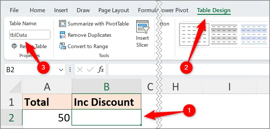
To apply a formula to an entire table column, simply enter the formula in any cell of the column. The table will copy the formula to all the cells of the column automatically.
The following formula is then used in column B (or the [Inc Discount] column).
=[@Total]*(1-$D$2)
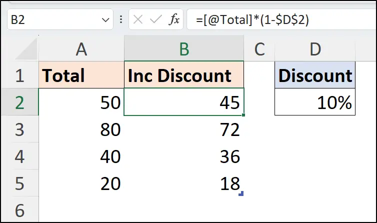
The structured reference [@Total] is entered by the table when cell A2 (or other cells in the column) are clicked. You can type it directly, but easier to let the table automatically enter it in this case.
With an Excel table, there is no need to copy a formula down a column. It is automatically filled by the table itself.
It also uses the same formula in each row, and if any formula in the column is changed, the formulas in the entire column are updated. I love this! Going beyond the grid with meaningful formulas and no double clicking the fill handle.
Learn how to apply absolute references to columns in an Excel table.
Using an Array Formula
Using a dynamic array formula to an entire column in Excel will ensure that the same formula is applied to each row of the range (array formulas cannot be used within Tables).
This technique uses one formula in a single cell as opposed to dragging the fill handle (or some other technique from this article) to copy formula down a column.
Using an array formula also removes the need for an absolute reference or named range to stop a cell changing when you copy a formula.
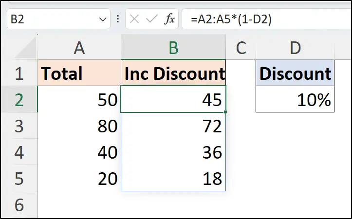
In this formula, you notice that the range A2:A5 has been used instead of the single cell A2, used in previous formula examples. This forces the formula to spill across multiple cells.
=A2:A5*(1-D2)
Wrap Up
This article detailed a variety of techniques to copy a formula down a column, and included Microsoft Excel tips to apply formula to other ranges too.
When working with tabular data, using an Excel table is really the way to go. The consistent formulas and automatic update of all formula to an entire column, are important benefits.
Understanding difference cell addresses such as relative and absolute is the most important technique to master. When to apply each technique and how to recognise them are an essential Excel skill.
Learn more than 150 of the best Excel functions in my Advanced Excel Formulas book. Over 500 Excel formula examples are demonstrated with practise files included.


Leave a Reply