Merge Queries in Power Query – VLOOKUP Alternative

In this blog post we explore how to replicate a VLOOKUP in Power Query using merge queries.

Excel users love VLOOKUP. It is one of the most useful functions there is. So it stands to reason that we may need to perform similar tasks in Power Query.

In this blog post we will look at performing common VLOOKUP scenarios by using merge queries within Power Query. And also discuss some of the differences (advantages of Power Query) between the two.

Advantages of using Power Query over VLOOKUP

Now Power Query may not always be the route I would take. Sometimes I just need quick answers. So I would bash out a quick VLOOKUP to get the results, and paste to values (if needed) to remove the formula.

Power Query has many advantages over the classic VLOOKUP function however. Simplifying tasks that with VLOOKUP would be awkward, or in some cases not possible.

Here are some of its advantages;

• Power Query can work with data from external sources directly (CSV files, databases, web queries) without first dumping the data into a worksheet. This can keep your workbooks lean and mean.
• In Power Query we could easily return multiple columns of data for the lookup value without the need for a separate VLOOKUP for each column.
• We can lookup based on multiple columns/conditions using the Power Query approach without needing complex array formulas or helper columns.
• Other steps could be added to Power Query to apply formatting, or remove bad rows.

Watch the Video

The Setup

Before we can perform the merge query, the ranges need to be formatted as tables (but lets be honest, they probably should be anyway).

If your data is not formatted as a table, Power Query will put it in one anyhow. So you don’t really get a choice.

You can do this by clicking in the range of cells, then click the Table button on the Insert tab of the Ribbon. You can then assign a name to the table on the Design tab.

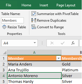
We then need to create our base queries. We cannot merge two queries, until we have them set up.

Please bear in mind, that although these examples use data on a worksheet.

A stronger example of Power Query in action would be when working with data from external sources. And in those situations, these queries would probably already exist.

Click a cell within one of the tables. Then click the Data tab and the From Table/Range button (these names may differ depending on your Excel version).

The Power Query Editor will open. The query can be named on the right side, otherwise the table name is used.

We do not want to do any editing yet. Click the drop arrow for the Close & Load button. Select Close & Load To.

The Import Data window opens. Select the Only Create Connection option.

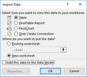
Repeat these steps for the other table.

These steps will also need to be performed as the foundation for all of the examples in this post.

Ok, with this now done, we can get on with some VLOOKUP scenarios.

Merge Queries in Power Query for a Simple Lookup

Let us start with the classic VLOOKUP. An exact match to return data from a lookup table into a main table.

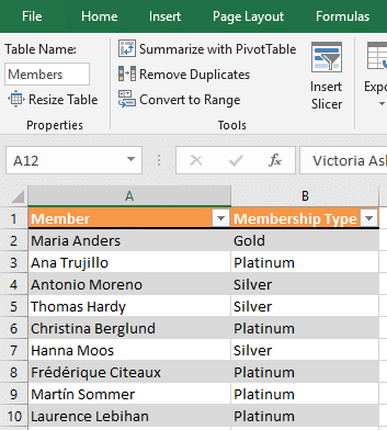
Take this example, where I have a table of members and their membership type. This table is named Members.

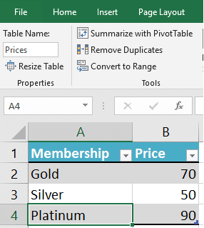
And another table which contains the membership types and their price. This table is named Prices.

You can download the merge-tables.xlsx file to follow this example.

We can start a merge query in a variety of ways. And some of these may differ depending on the version of Excel that you are using.

In this example, I shall click Data > Get Data > Combine Queries > Merge.

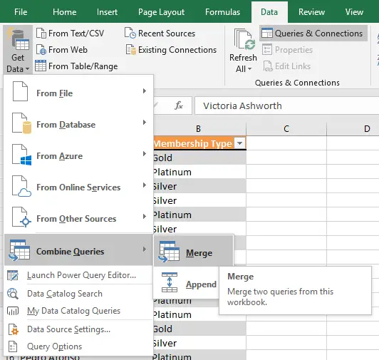
This will open the Merge Window. In the first drop list I will select the main table (Members) and then in the second list select the lookup table (Prices).

I then need to specify the columns from each table that I want to match. You can do that by clicking the column in each table, starting with the first table.

The Membership columns have been selected in this example.

Note that in the lookup table (Prices), the column we are looking in is the first one. But it could be any column of the table, unlike when using VLOOKUP.

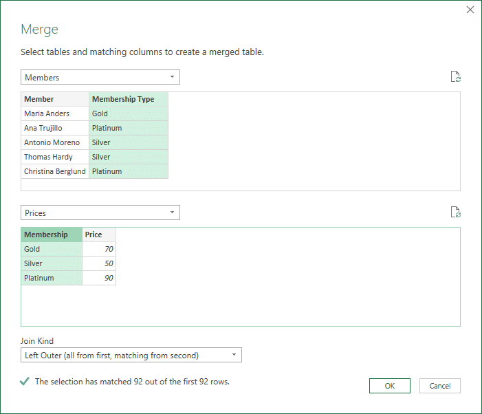
We then need to specify a Join Kind. There are 6 different join kinds, and I will talk more about these in the final example of this post.

For now, I will leave it as the Left Outer join kind. This is your typical VLOOKUP. It returns all the values from the main table, and only those that match from the second.

If it does not find a match, it returns a null value.

In this example, the message confirms that it has matched 92 out of 92 rows.

When you click Ok, you are taken to the Power Query Editor.

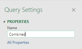
Enter a meaningful name for the query in the Query Settings pane on the right. This name will be used as the name of the table when loaded back into the workbook.

You will see a new column added to the table. It has a table icon in the header and the word table in every row.

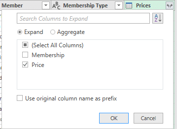
Click the button with 2 arrows in the column header to select which columns from the lookup table, you would like to import into the main table.

In this example I just want the Price column. Please note that you can select as many columns as you want (no need for multiple VLOOKUPs).

And I will definitely de-select the Use original column name as prefix option.

The column is successfully imported.

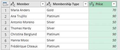
You can then perform more transformations using the magic of Power Query, but that goes beyond the purpose of this blog post.

Click the Close & Load button to load the table to a worksheet.

When data in either of the two tables changes in the future, the query can simply be refreshed by clicking the Refresh button on the Data tab.

Remember that although this example uses data on worksheets, these queries can be refreshed directly from an external source.

Multiple Condition Lookup with Power Query Merge Queries

One of the advantages of Power Query over VLOOKUP mentioned at the beginning of this blog post, was that it can return values when multiple conditions match.

So let’s have a look at an example.

You can download the merge-multiple-conditions.xlsx file to follow this example.

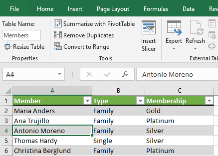
In this example, we have two tables. They are already formatted as tables, and the base queries have already been established.

Here is the Members table.

And here is the Prices table.

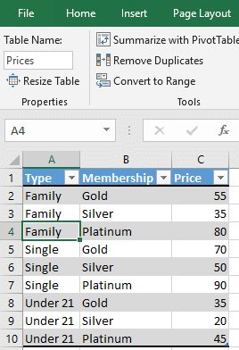
This time we want to return the Price column for when there is a match on the Type and Membership columns.

We can start a merge query and select the two tables in the Merge window by following the steps from the previous example.

When selecting the columns, this time we will select the Type column in each table. Then press down the Ctrl key on the keyboard, and select the Membership column in each table.

The result should be like the image below. A number appears next to each selected column. Ensure the numbers match in each table.

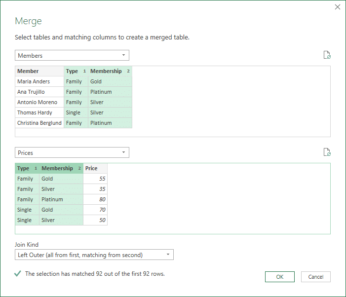
We will be doing a Left Outer join kind again.

Name the query, expand the table and select the Price column. Then close and load to the worksheet just like the previous example.

Comparing Two Lists using Other Join Types

Another very common reason to use VLOOKUP is to compare two lists.

You may want to know which items feature in one list, but not the other. Or which items appear on both lists.

Let’s look at how merge queries can achieve these tasks.

You can download the merge-tables-2.xlsx file to follow this example.

In this example we have 2 almost identical tables named MembersFirst and MembersSecond.

They are both formatted as tables already and queries created as connection only.

Here is one of those tables.

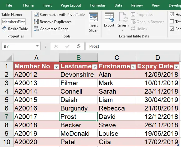
There are some members on both tables. Some on MembersFirst, but not on MembersSecond. And also some on MembersSecond, but not on MembersFirst.

We can begin the merge query like in the previous examples. Select both tables in the Merge window. And select the MemberNo columns in each table as the column to match records.

The difference this time is with the join kind that we select. When learning Power Query, it is important to get familiar with these different join kinds.

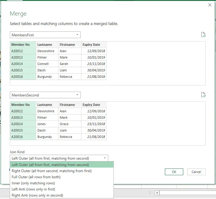
In this example, it is really the last four join kinds that interest us. And there is a decent description after the name of each join kind that probably explains it as well as I could.

Take the opportunity to try them all out and see what results you get.

In this example, I will choose the Inner join kind. This one will only return the members who appear in both lists.

Name the query as before, but this time we will not select any columns from the table in the fifth column. We are not interested in extra columns/fields as it is the same information that we already have.

What this has done though is only returned members that appear in both lists. In this example, that is 7 out of 9.

Click Close & Load to load the table into a worksheet.

That was our final example to show in this blog post. I highly recommend learning more about Power Query if it is new to you. It is an extremely powerful tool.