The IMAGE function in Excel enables us to return an image to a cell using an Excel formula.
This function makes it easy to lookup images based on a cell value, and because the image is stored in the cell, it is returned when sorting and filtering, and when using other functions such as XLOOKUP, FILTER and IF.
Excel IMAGE Function
The IMAGE function accepts five arguments, but only the source argument is mandatory. The other arguments enable us to specify alternative text and to specify the size of the image.
IMAGE(source, [alt_text], [sizing], [height], [width])- Source: The URL of the image file. This can be entered as a text string, be a reference to a cell containing the URL path, or be a formula that returns a valid URL path.
- Alt text: The alternative text for the image.
- Sizing: Determines the dimensions of the image. There are four options to choose from.
- 0 – used to fit the picture to the cell maintaining its aspect ratio.
- 1 – fill the cell ignoring the aspect ratio.
- 2 – keep the original image size even if it ignores the cell boundary.
- 3 – set the images height and width.
- Height: The image height in pixels.
- Weight: The image width in pixels.
The Excel IMAGE function can handle numerous image formats including JPEG, PNG, bitmap, TIFF, and more. The source, however, must be a URL using the ‘https’ protocol.
Download the practise workbook to follow along.
Let’s see some examples of it in action.
Insert Images in Excel using a Cell Value
I have some images stored on the Computergaga site. You can see the image URLs in the [URL] column of the table in the following image. This table is named Reps. We will return the image from that URL into the [Image] column.
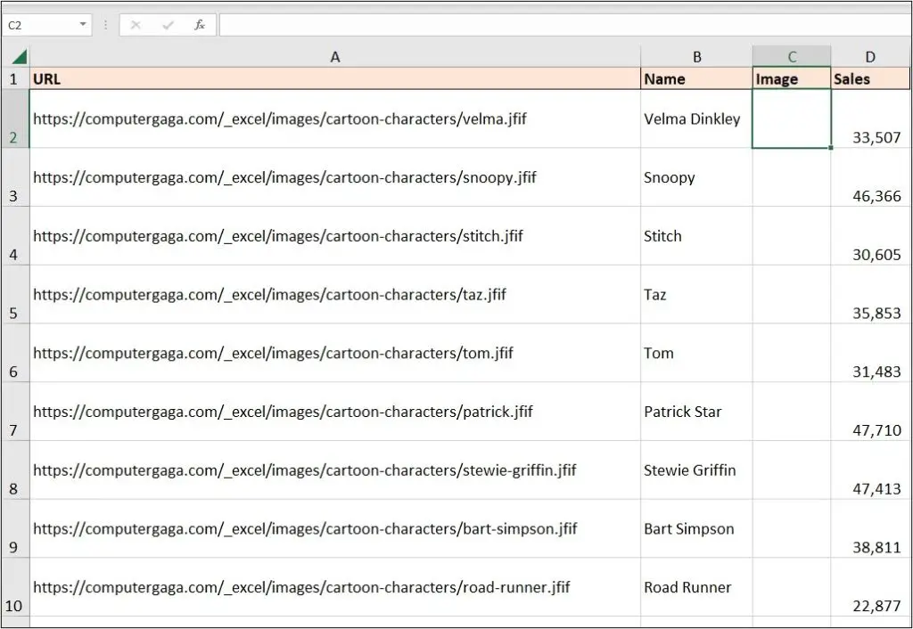
Using the Excel IMAGE function, it prompts for the five arguments and there are two main ways of specifying the “source”. One way is that we could enter it as a text string. This will work fine.
In the following formula, the URL for the Velma Dinkley image has been entered directly into the formula. This works perfectly fine as only that first argument is necessary.
=IMAGE("https://computergaga.com/_excel/images/cartoon-characters/velma.jfif")However, you can see that the same image has been returned for the entire table. This is because tables auto-complete a formula down the rows. The image returned doesn’t make sense in this example but it demonstrates the function working with that single piece of information and that it can be entered as a text string.
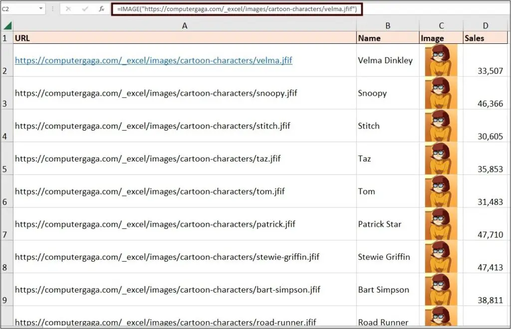
In this example, a far more effective formula would be to refer to the cell in the [URL] column of the table. This ensures that the formula returns the correct image for each row.
In the following formula, a reference to the [Name] column is made for the “alt_text” argument. You can type any text you want for the alternative text of an image. In this example, the text from the [Name] column works nicely.
The default value for the “sizing” argument (the third argument of the function) is 0, which fits the image to the cell. This maintains the aspect ratio. In the following IMAGE formula, a 0 has been entered, despite it being the default, therefore unnecessary.
=IMAGE([@URL], [@Name], 0)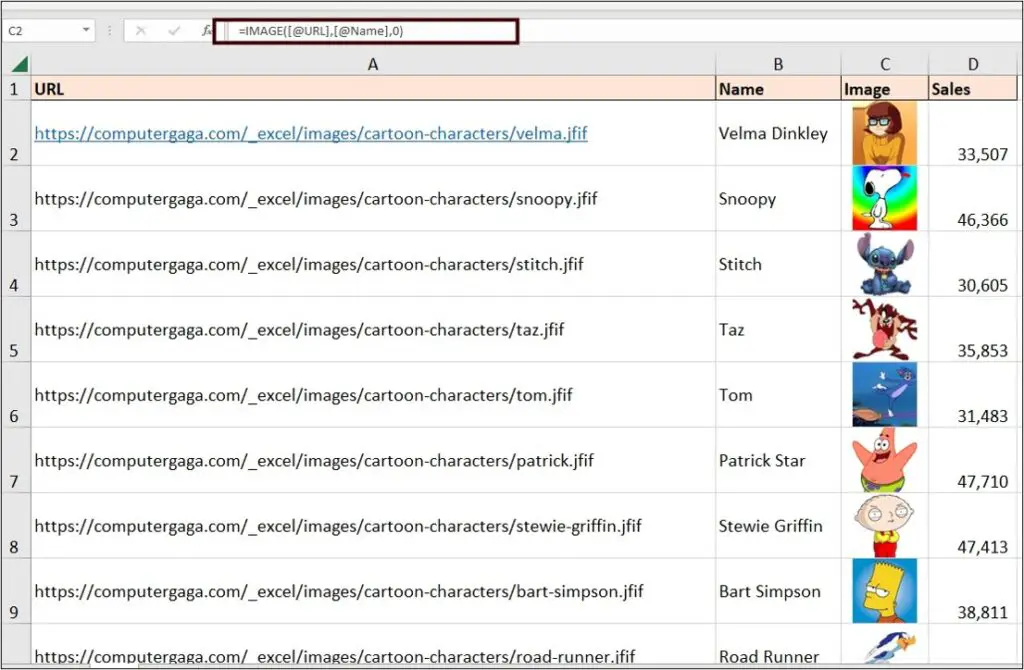
One simple formula to return an image for each member of the sales team, thanks to the Excel IMAGE function.
Sort and Filter Images in a Table
Because the IMAGE function inserts an image in the cell, the images will move when performing typical Excel tasks such as sorting and filtering a list.
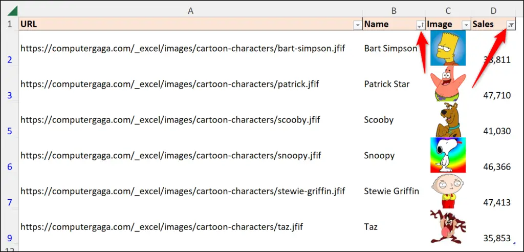
Select a cell in the [Name] column, go to the Data tab, and click Sort A to Z and the images will move with the other values in the row.
Click the filter arrow in the [Sales] column and set a filter for to show only those rows with a value greater than 35,000. The images are filtered along with other values in the row. How awesome!
The following image shows the resulting table ordered by name and filtered to only show rows where the sales value is greater than 35,000.
Excel Picture Lookup with IMAGE and XLOOKUP
In this example, I have a drop-down list in cell C3 with the names of all the sales staff in the “Reps” table, and when I select a name such as Bart Simpson, I want their image to be shown in cell D2 (the large merged cell with the border).
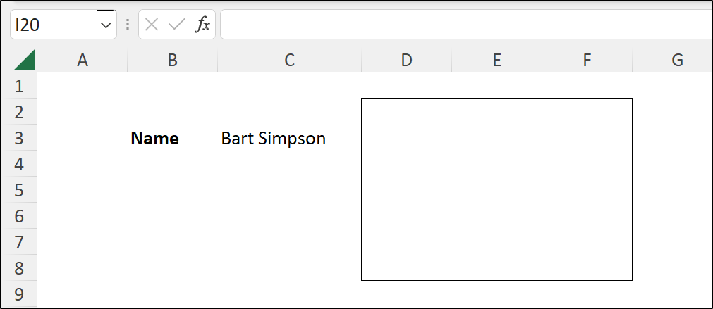
To do this, click on cell D2, and write the following IMAGE formula.
=IMAGE(XLOOKUP(C3,Reps[Name],Reps[URL]),C3,3,150,150)An XLOOKUP function is used for the ”source” argument of the Excel IMAGE function. XLOOKUP returns the URL from the “Reps” table where there is a match in the [Name] column for the name stated in cell C3.
The name in cell C3 is also used for the alternative text. And a custom size of 150 pixels in height and width was specified.
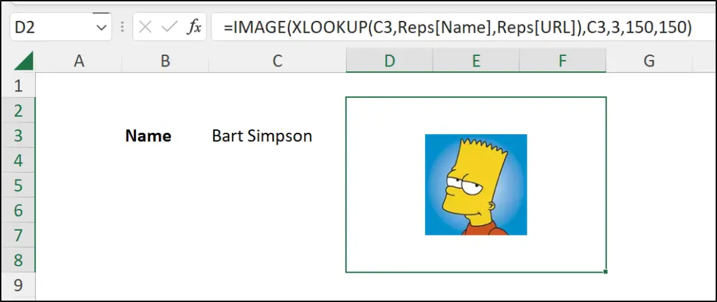
This formula returns the image based on a cell value dynamically. If a different name is selected from the drop down list, that picture is returned. It is a nice example of the IMAGE function in Excel being used with other Excel functions.
Return Images as Part of a Multi-Column Array
In this final example of the Excel IMAGE function, we are going to see images returned as part of a multiple column array.
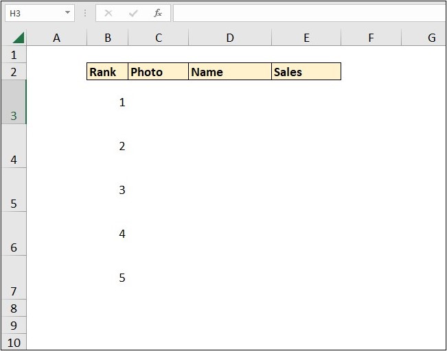
We will return the top five sales reps to cell C3 of the following image using a formula. I show a few examples in my Advanced Excel formulas book of how to calculate rankings and create top N and bottom N lists, but for this example in cell C3, we are going to use the SORT function to sort the “Reps” table by column four (the [Sales] column) in a descending order. We will then take only the top five rows from the returned table.
The following formula uses the SORT function to return all columns of the “Reps” table in descending order by column four (this is the [Sales] column of the “Reps” table).
=SORT(Reps,4,-1)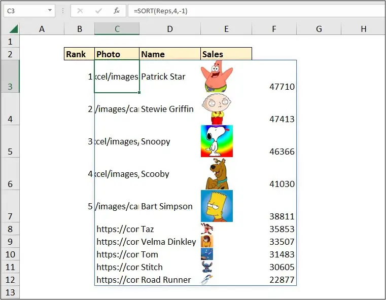
The SORT function results look ugly as we have the URL in the first column instead of the images, and we have different size images as they are being fit to the cell.
In the following formula, the CHOOSECOLS function has been added to specify the columns that we want, and in the order we want them. With CHOOSECOLS, columns 3 (Image), 2 (name), and 4 (sales) have been returned in that order.
=CHOOSECOLS(SORT(Reps,4,-1),3,2,4)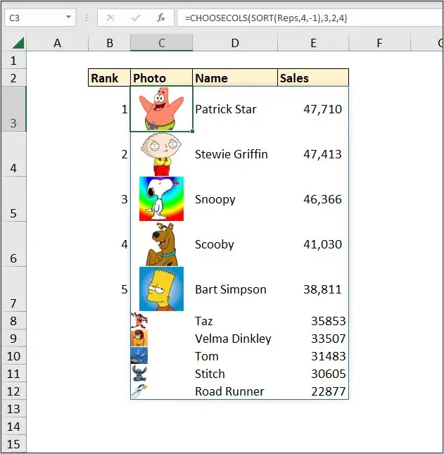
Finally, the TAKE function is added to return the first 5 rows only.
=TAKE(CHOOSECOLS(SORT(Reps,4,-1),3,2,4),5)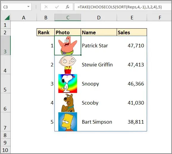
The real purpose of this example is to show the images being returned as part of multi-row and multi-column spill range. There are many examples of how useful the Excel IMAGE function is for our reports and other tasks that you are accomplishing with Excel that involve images.
What do you think? Do you have a need for the IMAGE function in Excel? Let us know in the comments.



Leave a Reply