Essential Conditional Formatting Tricks

Conditional Formatting is an amazing feature of Excel. It is sure to create a spark of interest and questions during training. People see the potential in their spreadsheets and how easy their team could visualise their data and create engaging reports.

This tutorial looks at the two most requested Conditional Formatting tricks asked by Excel users.

Download the file used in this video to follow along.

How to Format the Entire Row

Formatting a cell is great, but what if your data is many columns wide. Applying Conditional Formatting to the entire row will be far more effective in spreadsheets that have many columns.

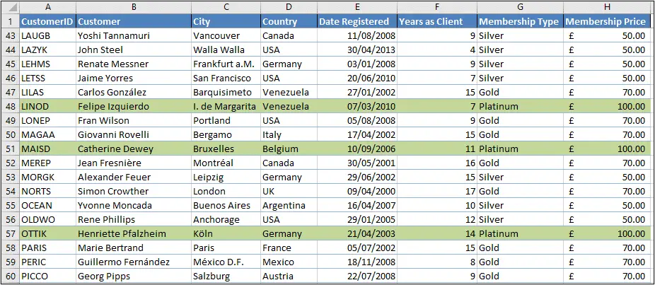
For example, in the spreadsheet below I formatted the entire row where the membership in column G is Platinum.

1. Select the entire table of data excluding the header row.
2. Click the Home tab on the Ribbon and then the Conditional Formatting button.
3. Select New Rule from the list.
4. Click on Use a formula to determine which cells to format in the top half of the screen.
5. Enter the required formula in the Format values where this formula is true box.

The following formula was used to reference a different cell to the one being formatted. The mixed reference (column is fixed, but row is relative) of $G2 is used to check down column G, but not across the columns.

=$G2="Platinum"

6. Click the Format button and choose the formatting you would like to apply.
7. Click Ok.

How to Use Multiple Conditions in your Conditional Formatting Rules

The Conditional Formatting tool makes it easy to set up simple conditional rules. These may be Ok for most of your needs.

The second of our essential Conditional Formatting tricks takes things a step further and uses multiple conditions for a rule.

To use multiple conditions in Conditional Formatting you will need to enter a formula. Depending on the logic you want to use this will likely be either the AND or OR function  (Find out more on the AND and OR functions in Excel).

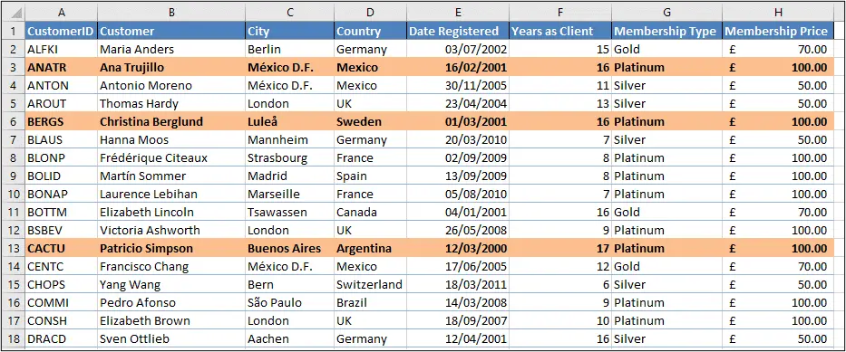
For example, in the image below I have formatted the entire row where the customer has been with use for 10 years or more, and they have a Platinum membership.

1. Select the range of cells you want to apply the Conditional Formatting to.
2. Click the Home tab on the Ribbon and then the Conditional Formatting button.
3. Select New Rule from the list.
4. Click on Use a formula to determine which cells to format in the top half of the screen.
5. Enter the required formula in the Format values where this formula is true box.

The formula below uses the AND function to ensure that both conditions are met.

=AND($F2>=10,$G2="Platinum")

6. Click the Format button and choose the formatting you would like to apply.
7. Click Ok.

There is no limit to how complex this criteria may be. Conditional Formatting rules can be created to meet your needs whatever they may be, you just need to know the formulas you need to use.

Other Conditional Formatting Tricks

• Highlight dates over 30 days old
• Conditional Formatting with charts
• Highlight Saturday and Sunday in a list
• Using Conditional Formatting with PivotTables

Please share your own favourite Conditional Formatting tricks by commenting on this post below.