Create a Scrollable Chart for your Excel Dashboards

Creating a scrollable chart in Excel is a great chart trick for enhancing the functionality of your Excel dashboards. You may have years of data to display in the chart, and yet space is limited on your spreadsheet.

By adding a scroll bar to the chart, users can interact with the chart and scroll to see the data they want displayed.

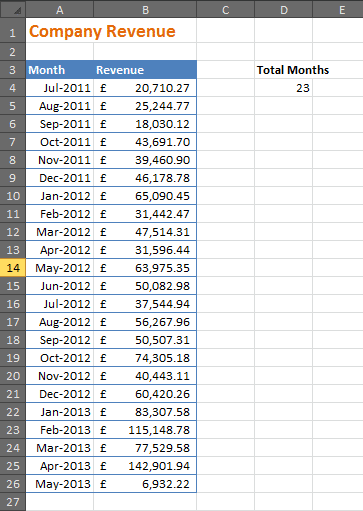
In this example, we have a spreadsheet with revenue for the last 23 months. As this is a lot of data to plot, we have decided that the chart will only display 5 months at a time. A scroll bar will be added so that users can scroll through the years.

Skip to watching the video.

Create a Scrollable chart in Excel

The screenshot below shows the 23 months of revenue on the spreadsheet.

Download the spreadsheet to follow along

Use the INDEX Function to Prepare the Source Data

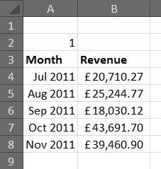
Our first task will be to create a condensed version of this table only showing the 5 months that the chart will use as its source.

1. On a new worksheet, enter 1 in cell A2. The reason for this number will become clearer as we go on. Essentially this value will change as the user scrolls on the chart. It stores the row number of the data to return for the chart.
2. Write the following the INDEX function in cell A4.

=INDEX('All Data'!$A4:$A$26,Chart!$A$2)

The INDEX function is used in Excel to return a value from a specified row and column. Its syntax is;

=INDEX(array, row_num, [column_num])

In this instance we are using it to return the value from column A that is in the row number stored in cell A2 of the Chart sheet.

There is no dollar sign before row 4 in the formula. This is important, as it ensures that when we copy the formula down, the row number will change. All other parts of the reference are fixed.

3. Copy the formula down to cell A8.
4. Enter the formula below in cell B4.

=INDEX('All Data'!$B4:$B$26,Chart!$A$2)

5. Copy the formula down to cell B8.

Create the Chart

Now that we have the data source, its time to create the chart.

6. Select range A3:B8.
7. Click the Insert tab, Line and select a Line graph.
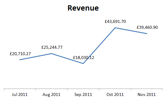
8. Perform any formatting options you want for better presentation. In the example below I have removed the Legend, removed the value axis and gridlines, and also added the values as data labels to the chart.

Add the Scroll Bar to the Chart

The final stage and the one we have been waiting for is to add the scrollbar to the chart.

9. Click the Developer tab on the Ribbon.

Note: If the Developer tab is not visible, click File > Options > Customize Ribbon and check the Developer box on the right.

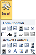
10. Click the Insert button and select the Scroll Bar ( Form Control) from the menu.

10. Click and drag to draw the scroll bar onto the worksheet underneath the chart.
11. Click on the Properties button on the Developer tab, or right mouse click the scroll bar and select Format Control.
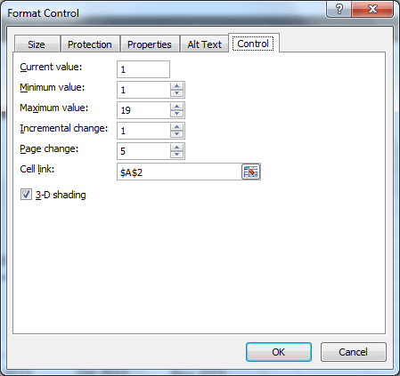
12. The Format Control dialog box opens. Ensure the Control tab is selected.
13. Enter 1 in the Current value field.
14. Type 1 for the Minimum value. The lowest row number in the table is number 1.
15. Enter 19 for the Maximum value. There are 23 months of data. By displaying 5 months on the chart at any time the maximum row number must be 19.
16. Type 1 for the Incremental change. This is the number of months the chart scrolls when the scroll bar arrow are clicked.
17. Enter 5 in the Page change field. This is the number of months that the chart scrolls when you click within the scroll bar.
18. Click in the Cell link field and then select cell A2 on the sheet. The reference $A$2 should appear in the field. This is the cell containing the row number to return for the chart. The scroll bar will change this when used.

20. Click Ok.

Click elsewhere on the spreadsheet to make the scroll bar active. Now when used  the chart changes the information that is displayed.

Watch the Video – Scrollable Chart in Excel