Create a Searchable Drop Down in Excel – Just Like Google Search

This blog post will take you through the steps to create a searchable drop down list in Excel – just like Google search.

This is a great Excel trick for working with large drop down lists.

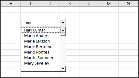
In this tutorial we will use a list of 87 names that as we type into the drop down list, it searches the names, and the list shortens to show only those names containing that string of characters.

There are a few formulas to write to get this searchable drop down list in Excel created. Everything is shown and provided in this tutorial. If you prefer a video. Check out the video tutorial below.

Watch the Video – Searchable Drop Down List in Excel

Modern Excel – Easier Method

If you are using an Excel 365 or Excel 2021 version of Excel, then this much easier method is possible. The dynamic array engine in modern Excel has greatly eased the process to create a searchable drop down list in Excel.

Do not have an Excel 365 version? Please read on or watch the previous video.

Create the Combo Box Control

The drop down list used here is the combo box control. It is not a Data Validation list. So the first task is to insert a combo box control where you want the list to be.

1. Click the Developer tab on the Ribbon (don’t have a Developer tab? Right click the Ribbon, select Customise the Ribbon and check the Developer on the right).
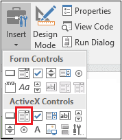
2. Click the Insert button in the Controls group and select the Combo Box (ActiveX Control).

3. Click and drag to draw this control onto the worksheet. You can always move and resize the control later, so don’t worry about 100% accuracy.
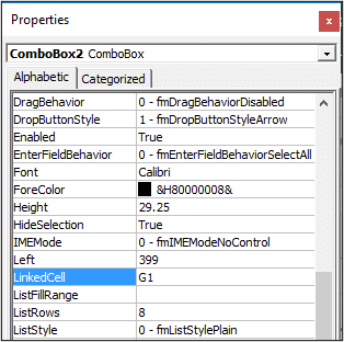
4. Now we need to link the combo box value to a cell. After inserting the combo box, you should already be in design mode. Click the Properties button on the Developer tab. If this is not active, click the Design Mode button and then Properties.
5. The Properties window appears. In the LinkedCell property, type the cell address of the cell you want the combo box linked to.

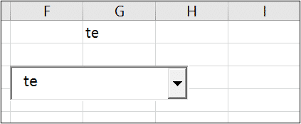
6. Let’s check out what we currently have. Click the Design Mode button to exit design mode. Type into the combo box and you should see the value appearing in the cell you linked it to.

Identify Which Names Contain the Characters being Searched for

To be able to create this searchable list, the first formula will need to identify which names meet the criteria and should continue to appear in the list when the user is typing.

To identify the names that contain the characters being searched for, we will use an Excel function with a very appropriate name – the SEARCH function.

The SEARCH function below can be used.

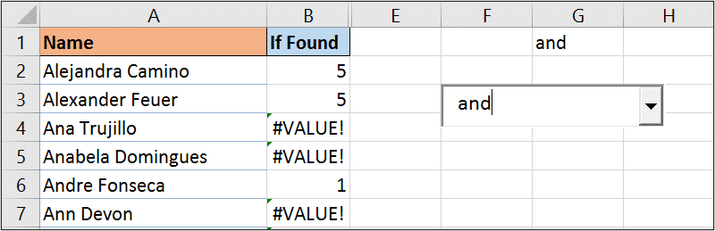
=SEARCH($G$1,A2)

In this function, cell $G$1 is the cell that the combo box is linked to. So this contains the string of characters that we are looking for. Cell A2 is the first name in the list of names.

This function will return the #VALUE! error if a name does not contain the characters typed, and returns the first occurrence of those characters if it does.

In the image below you can see that the characters being searched occur in the fifth position of the names in A2 and A3, in position 1 of A6 and not at all in the other cells.

Now this is what we need. We now know which names should be appearing in the final drop down list while users are searching.

However, I don’t like the #VALUE! error and I’m not really interested in what position the characters are in. I just need to know that they are there.

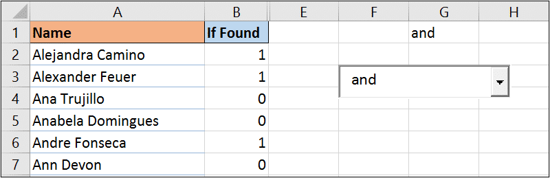
The ISNUMBER function can then be added to the SEARCH function so that it returns TRUE or FALSE when a name is identified or not. The double negative is then added before the ISNUMBER function to convert the TRUE or FALSE to 1 or 0.

=--ISNUMBER(SEARCH($G$1,A2))

How Many Names Contain those Characters

The next formula needs to count how many names in the list contain the characters being searched for.

This is important to create the dynamic aspect of the searchable drop down list. As characters are typed the list should shrink, and then expand again when the characters are deleted.

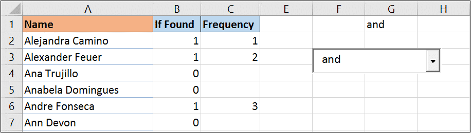
The COUNTIF function is used here to count the occurrences of names being returned. This function uses a reference to the ‘IF Found’ column in B. It has a fixed start point of $B$2, but a relative row number on the end point $B2. This ensures that the reference gets bigger as the formula is copied down.

It is counting how many times a 1 occurs in the range up to the point of the current row.

COUNTIF($B$2:$B2,1)

An IF function can then be added to it so that it only performs the COUNTIF, if the cell contains a 1, otherwise show blank in the cell.

=IF(B2=1,COUNTIF($B$2:$B2,1),"")

Return the Names for the Searchable Drop Down List

We now know which names should be appearing in the list, and we also know how many there are.

Next step is to create a range of cells containing these names only. A drop down list can then use this range of cells.
To lookup these names we can use the amazing INDEX and MATCH function combination.

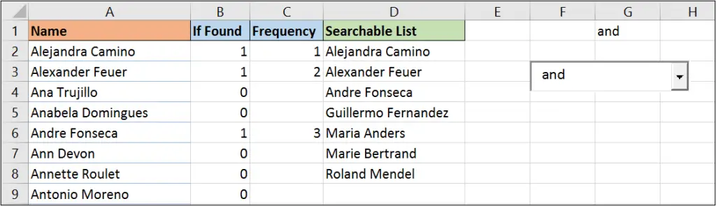
=INDEX($A$2:$A$88,MATCH(ROWS($C$2:$C2),$C$2:$C$88,0))

The INDEX function is used here to return a name from the range A2:A88  from the row specified by the MATCH function.

The ROWS function is used to return the current row number. So for the first name in the list it is row 1 of that range. The second name is row 2 and so on. This works to provide MATCH with the current name we are looking for (1st, 2nd etc).

The MATCH function then looks for this number in range C2:C88. It reports back to INDEX with the names position, and INDEX extracts the name.

The IFERROR function can then be added to this so that the cell contains blank if there are no more names to look for.

=IFERROR(INDEX($A$2:$A$88,MATCH(ROWS($C$2:$C2),$C$2:$C$88,0)),"")

Define a Dynamic Named Range for the Searchable List

Now that we have the returned names, we need an easy way of referring to them. For this we will create a named range. This will need to be dynamic and detect how many names are returned. The combo box will then use this named range for its list.

Click the Formulas tab on the Ribbon and then Define Name. Enter a name for the range (I named it employees) and then enter the formula like below into the Refers to field.

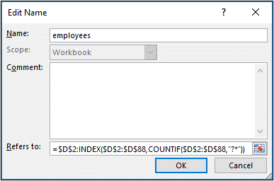
=$D$2:INDEX($D$2:$D$88,COUNTIF($D$2:$D$88,"?*"))

To create the dynamic named range we used the INDEX function with COUNTIF. The INDEX function is capable of returning a value or a reference and in this scenario we need it for the latter.

The dynamic range starts from $D$2 and then the COUNTIF function is used to locate the last name in the list for the INDEX function. The “?*” is used as the criteria to count the number of cells containing text.

Assign the Dynamic Named Range to the Combo Box

Now that we have the searchable list of names in a column and the range has been named. The combo box needs to be told to use this named range as its source.

1. Click the Developer tab on the Ribbon and then the Design Mode button.
2. Now we are in design mode, click on the combo box control and then click the Properties button.
3. Type the name that you gave your named range into the ListFillRange field.

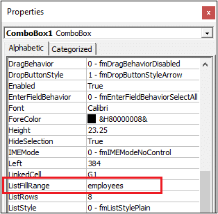
4. Close the properties window.

Make the List Drop Down on Change

The final step is to make sure the list drops down when somebody types into it. At the moment someone could click the list arrow to drop it down, but if they type, no list appears.

1. Double click on the combo box (you need to still be in design mode for this).
2. This will take you to a code window to enter a tiny piece of VBA code. Type the line below in between the Private Sub and End Sub lines.

Private Sub ComboBox1_Change()
ComboBox1.DropDown
End Sub

Adjust the Combobox1 part to the name of your combo box.

If you are interested in learning VBA then check out our Excel VBA online course. It is a fantastic skill to have if you are a heavy Excel user.

Exit design mode and test out your combo box. You should now have a searchable drop down list to use on your Excel reports, dashboards and forms. Everyone will be asking how you did it.

More Excel Tutorials

• Create a picture lookup in Excel
• Excel formula to find the least frequent value
• Awesome scrollable chart for your Excel dashboards
• Compare two lists and highlight matched items