Combine Multiple Worksheets into One with Append Query

One of the most common questions to receive in training is to consolidate or to combine multiple worksheets into one.

The best options available to do this are the Get and Transform features of Excel (known as Power Query in previous versions), or to create a macro using VBA.

In this blog post we will explore the Append Query feature of Get & Transform.

We have a workbook which contains 4 worksheets named France, UK, Spain and Italy. Each one contains sales data. The scenario is to combine these into a single worksheet for analysis.

We want to imagine that this is a regular process (maybe weekly). This data is downloaded or received in some way from an external source. And it needs to be combined into one worksheet quickly and easily.

Combine Multiple Worksheets with the Append Query

The Get and Transform features of Excel are truly incredible and more than up for the task of achieving what we need here (Learn more about Get and Transform in Excel)

For this demonstration, the data on each worksheet is formatted as a table. This is not necessary, but is advantageous.

One of the advantages is that when new data is added to the worksheets, the table will automatically expand.

Once we have combined all the worksheets with the Append Query. It can be refreshed in the future at the click of a button. So by having the data in tables, it is more dynamic and reliable.

You can watch this process in the video below.

1. Clicking in your range of data.
2. Clicking Home, Format as Table and selecting a style.
3. Ensure the range is correct and click Ok.

With the data from each worksheet formatted as a table, we now need to create a separate query for each one.

Please remember that you will not need to do these steps each week, or other time the data is changed. Once the queries are created, in the future we just press a button.

To create the queries;

1. Click in the table, and click the Data tab and then From Table/Range (depending on your Excel version, some of these steps may look a little different).

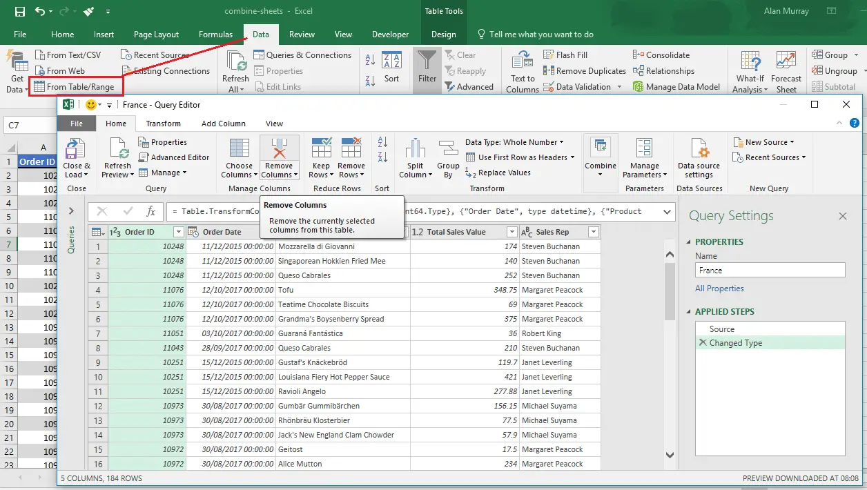
2. You can name the query in the settings on the right. By default is takes the name of the table. In this example, that is perfect. Click the Close & Load drop arrow, and select Close & Load To.
3. Select Only create connection and click Ok.

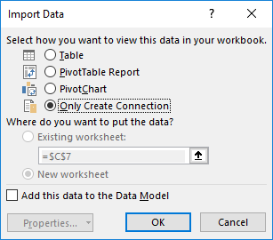
4. Repeat these steps for each worksheet/table.

When complete you will see each query in the Queries and Connections pane on the right.

Now to combine multiple worksheets data together by appending the queries.

1. Click Data > Get Data > Combine Queries > Append (remember your steps may be a little different).

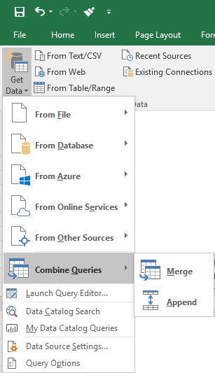
2. The Append window appears. We now need to select all the tables we want to append. Because we have 4, we need to select the Three or more tables option.
3. Select all 4 tables in the list on the left by clicking the first, and holding Shift and clicking the last. Then click Add to copy them to the list on the right. And click Ok.

4. The Query Editor window will load showing the appended tables. Change the name of the Query in the Query Settings window on the right. In this example, it has been named all-countries.

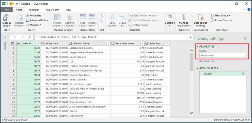
5. Click the Close and Load button to load it into a new worksheet.

A new worksheet is created with the combined data from all of those sheets.

The query has also been added to the Queries & Connections pane on the right. You can see the number of rows that was loaded here.

If the data on any of the tables change. This combined list can be updated simply by clicking the Data tab and the Refresh All button.

Now that you have learnt the Append query, check out Merge queries in Power Query. Incredible feature.