Aggregate Rows in Power Query

There are two main reasons you should consider aggregating rows in Power Query: creating a pivot-style report or reducing the number of rows and the granularity of your data without writing complex formulas.

This tutorial will teach you how to aggregate rows in Power Query, exploring how to aggregate both numeric and text values.

Download the practice file to follow along.

Take these Steps to Aggregate Rows in Power Query:

The option to aggregate rows in Power Query occurs in two main situations:

• When expanding a table in Power Query. For example, as the result of importing data, or the result of a merge query.
• When you use the Group By feature of Power Query.

Let’s explore aggregating rows with the Group By feature.

Step 1: Import Multiple Tables from Excel

We are going to import our sample data into Excel via an external connection. The sample Excel workbook contains four worksheets. Each containing tables with similar column headers.

To import the sample data, follow these steps:

• Open a blank Excel workbook.
• Navigate to the Data tab.
• Click on the Get Data dropdown > From File.
• Choose From Excel Workbook. Your computer’s library will open, allowing you to select and import the Excel workbook.
• Select the folder and click on Transform Data in the Navigator window to load the entire data into Power Query.

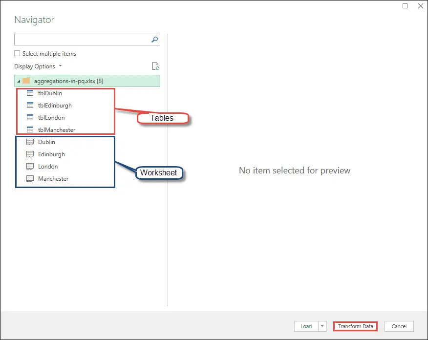
This will load your data into the Power Query window to transform the query – rename, filter and remove unwanted columns.

To apply the mentioned transformations, follow these steps: 

1. Rename the query:

• Right-click on the query in the Queries pane.
• Choose Rename from the menu that appears.
• Edit the query name.

2. Filter tables:

• Click the drop-down arrow in the [Kind] column header.
• Uncheck Sheet and click OK.

3. Remove other columns:

• Select the [Name] and [Data] columns.
• Right-click and choose Remove Other Columns.

4. Replace prefix:

• Select the [Name] column.
• Go to Replace Values in the Transform group, to remove the tbl prefix before each table.

The final result will display the names of the locations and the tables associated with each location.

Note that the name of the location corresponds to the different Tables in the workbook.

Step 2: Expand table structures

To perform any grouping, we need to expand the table structures in our data. This will display the initial base table data. 

To do this, follow these steps:

• Click the button in the [Data] column header.
• Choose Expand.
• Uncheck the Use original column name as prefix.
• Click OK.

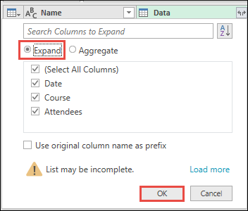
The table will expand. Ensure that you set the correct data type for each column header.

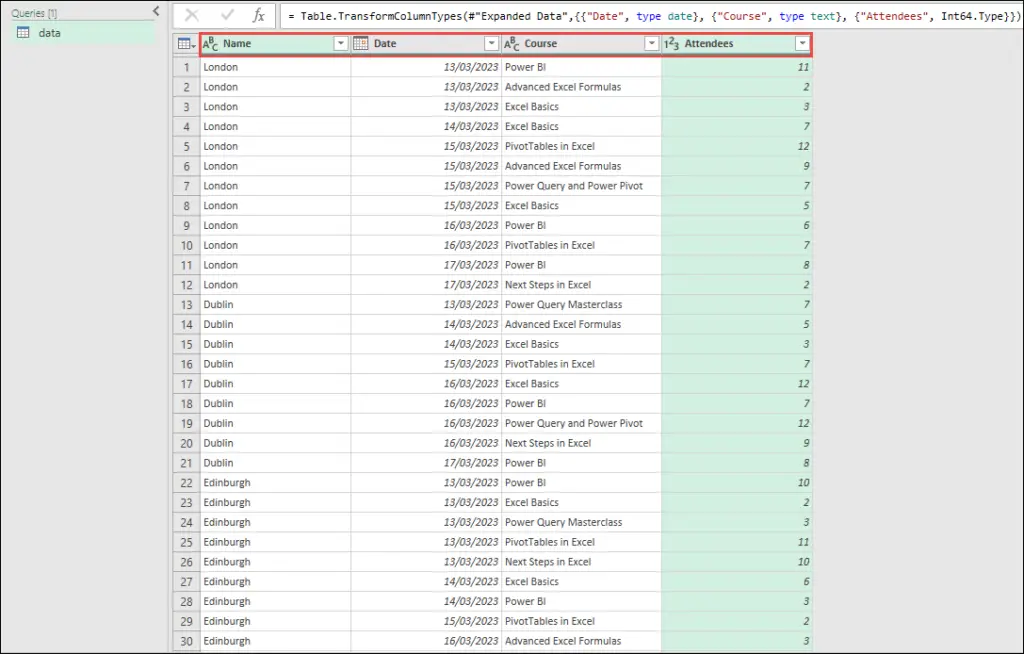
Basic Group By in Power Query

A basic group by allows us to specify a single column.

To demonstrate this, we are going to create a report for the number of attendees for each of the courses offered across all dates and locations. This is similar to what can be done with a pivot table or by loading the data as a table and using formulas such as SUMIFS or SORT. Let’s see how to do this in Power Query.

To group by course, follow these steps:

• Select the [Course] column.
• Click the Group By button in the Transform group.

This will open the Basic edition in the Group By dialogue box. Usually, the column selected will be included in the group by field by default. You can also specify another column if needed.

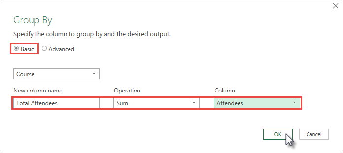
• Enter “Total Attendees” as the new column name for the aggregated values in the New column name field. 
• Select Sum as the aggregation function from the drop-down under Operation. 
• Choose the [Attendees] column from the drop-down under Column. 
• Click OK.

This will provide a report showing the total attendees on each course.

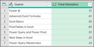
Note: To perform basic or advanced grouping, we reference the initial base data query and renamed the queries By Course and By Location and Date. This ensures that any changes in the main data table will be reflected in the referenced query.

Advanced Group By in Power Query

The advanced group by functionality in Power Query allows you to group by multiple columns simultaneously. In this example, we will demonstrate grouping based on the locations and dates for each of the courses.

To group by location and date, follow these steps:

• Select the [Name] and the [Date] columns. The [Name] column is the same as the location.
• Navigate to the Home tab.
• Click Group By in the Transform group. This will open the Advanced edition in the Group By dialogue box.
• Enter “Total Attendees” as the new column name under the New column name field.
• Select Sum as the aggregation function under Operation.
• Choose the [Attendees] column as the aggregation column.

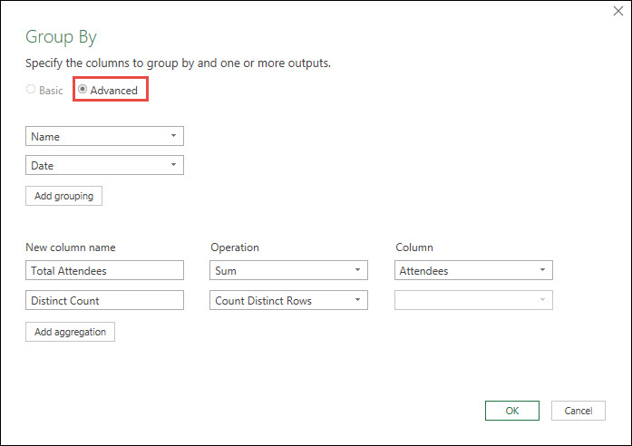
To add another aggregated column for Distinct Counts:

• Click Add aggregation.
• Enter “Distinct Count” in the New column name field.
• Choose Count Distinct Rows from the drop-down list under Operation.
• Click OK.

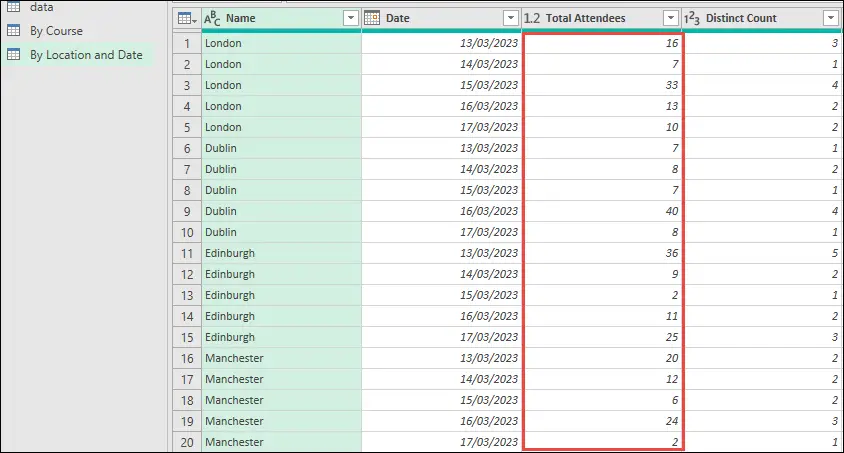
This will generate a report displaying the total attendees for all the courses covered in a specific location on a given date. Columns are added to aggregate rows by sum and a distinct count.

Aggregate Rows with Text in Power Query

So far, we have focused on aggregating numeric values. Now, let’s explore how to aggregate text values.

Here, we want to add a column to the previous query to determine the courses covered in each location on the same date.

Since there is no specific text function available in the Operation drop-down menu, such as CONCATENATE or TEXTJOIN, we will need to modify the M code through the formula bar.

To aggregate text, follow these steps:

• Click on the Gear icon next to Grouped Rows in the Applied Steps pane.

The Group By dialogue will reopen, allowing you to make changes to the applied step.

• Click Add aggregation.
•  In the New column name field, enter “Course.”
• Choose Sum under Operation.
• Select the [Course] column from the Column drop-down list.
• Click OK.

This will produce errors in the aggregated [Course] column as the Sum function cannot be directly applied to text values.

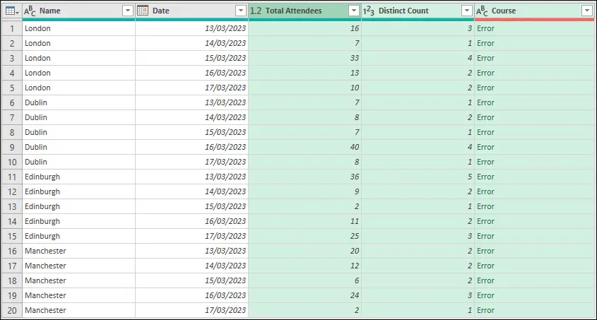
To correct these errors, you will need to edit the M code by following these steps:

• Go to the Formula bar in Power Query. 
• Select List.Sum and replace it with Text.Combine.
• Enter a comma after [Course] to move to the second argument of the Text.Combine function.
• Enter “,” to add a comma as the separator for each course.
• Click outside of the formula bar to apply the changes.

The edited M code should appear as follows:

Text.Combine([Course], ",")

After implementing this modification, each row will display a list of the courses happening on the same date and location.

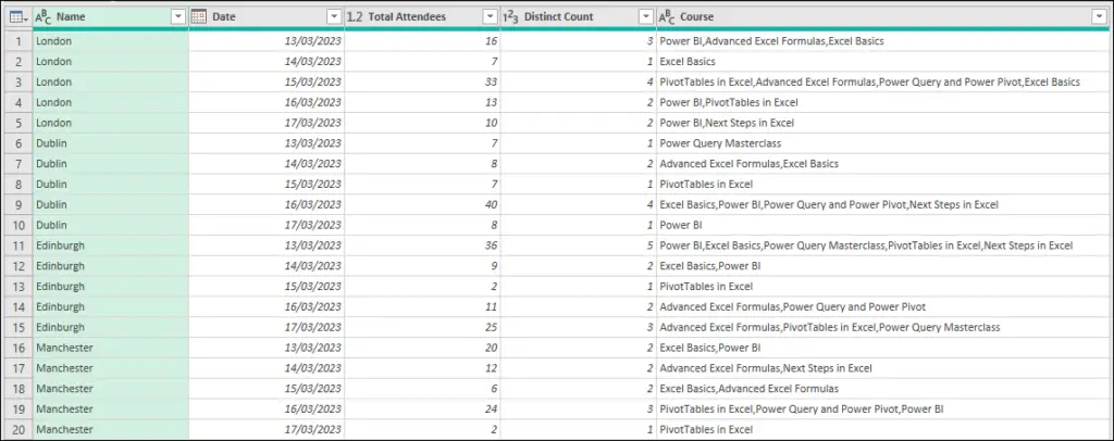
Bonus: Notice the gear icon on the Applied Steps pane no longer exists. This means that you can no longer edit this window as Text.Combine was not an option available in the Group By window.

Load to Excel as separate tables on the same sheet

Now it’s time to load our aggregated report into the Excel workbook. We will load the two reports as separate tables within the same worksheet.

The default load destination in Power Query is to load as tables on different worksheets. To change this, we will load the queries as Connection Only, and then edit this to load as a table on the Excel sheet.

To accomplish this, follow these steps:

• Navigate to the Home tab.
• Click on Close and Load To.

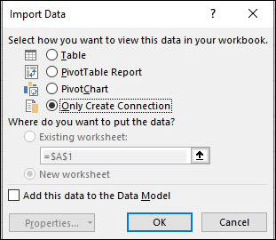
The Import Data window will open.

• Click on Only Create Connection since we only want to create a connection to the data without loading the original data table.

The Queries & Connections pane will open on the right side of your Excel sheet.

• Right-click on the By Course query.
• Select Load to from the menu. This reopens the Import Data window.
• Choose Table and specify a cell on the worksheet to load to.
• Click OK to load the data into the selected cell within the worksheet.

By following these steps, you can effectively aggregate rows in Power Query, create insightful reports, and reduce data granularity without the need for complex formulas.

I hope this information proves helpful. Let me know in the comments!