Advanced SUM Function Examples – The Power of SUM

This tutorial shows some advanced SUM function examples. The SUM function is far more powerful than many people realise, and this tutorial will demonstrate its power.

We will see five examples of the SUM function being a BOSS and handling tasks that we often rely on functions such as SUMIFS, XLOOKUP, SUMPRODUCT etc to accomplish.

However, trusty old SUM can take care of them alone.

Download the Excel workbook to follow along.

Sum Multiple Criteria with OR Logic

In this first example, we need to sum the values dependent upon two criteria from the same column. For this, we need to use OR logic with the two criteria.

We have a table named tblSales and need to return the sum of the Total column for sales of the products “Burger” and “Pizza”, entered into cells E3 and F3 respectively.

The following SUM formula entered into cell G3 accomplishes this easily.

=SUM(tblSales[Total]*(tblSales[Product]=E3:F3))

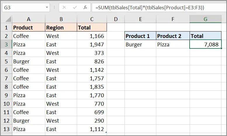
It takes full advantage of the array engine built into modern Excel versions, and multiplies the array of total values by the array of TRUE or FALSE responses from the condition. Watch the video for a more detailed breakdown of this behaviour.

If you are using an older version of Excel, e.g., Excel 2010, 2013, 2016 or 2019. Then instead of pressing Enter to run the formula, press Ctrl + Shift + Enter. This runs an array formula in older Excel versions.

This concise little formula is a fantastic alternative to writing two SUMIFS functions and adding them together like the following.

=SUMIFS(tblSales[Total],tblSales[Product],E3)+SUMIFS(tblSales[Total],tblSales[Product],F3) 

Or using the brilliant SUMPRODUCT function. However, It is great to see the classic SUM function handling this task on its own.

Advanced SUM Function with OR and AND Conditions

It is only a small step from the previous function to sum values that include both AND and OR logic in its multiple criteria.

With the same table (tblSales), this formula sums the values for both the “Burger” and “Pizza” sales for only the region of the “West”. The following advanced sum formula is entered into cell E6.

=SUM(tblSales2[Total]*(tblSales2[Product]=E3:F3)*(tblSales2[Region]=G3))

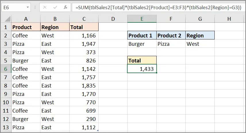
The asterisk (*) is used to create AND logic between the two sets of conditions.

Users of the SUMPRODUCT and FILTER functions of Excel will be familiar with this behaviour. Although they may not have done it with SUM before.

Two-Way Lookup with the SUM Function

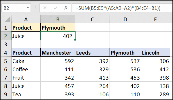
The SUM function can even perform lookups. Now, it can only return numeric values, not text, because of its sum behaviour. But it is pretty awesome.

The following formula is used in cell B2 to look up the value for the product in cell A2 (Juice) and the location in cell B1 (Plymouth).

=SUM(B5:E9*(A5:A9=A2)*(B4:E4=B1))

This SUM formula is more concise than some of its lookup counterparts.

For example, the INDEX and double MATCH formula approach would look like this.

=INDEX(B5:E9,MATCH(A2,A5:A9,0),MATCH(B1,B4:E4,0))

Now, I consider the INDEX function to be one of the best in Excel, so this is no slight on that function, but the SUM alternative is simpler in this instance.

How about a double XLOOKUP to create a two way lookup.

=XLOOKUP(B1,B4:E4,XLOOKUP(A2,A5:A9,B5:E9))

These array formulas are great fun.

SUM IFS with Lookup

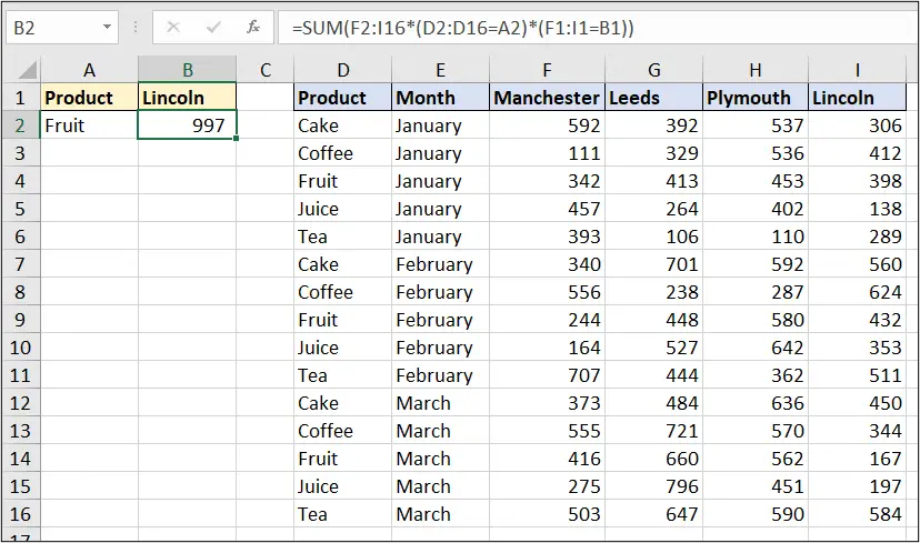
Following on from the previous example, if the product name occurred multiple times than the SUM function would perform its primary job of summing values.

So, this example is behaving like a SUMIFS function would for the conditional sum of the product, but with the column of values to sum being based on a cell value.

=SUM(F2:I16*(D2:D16=A2)*(F1:I1=B1))

Weighted Average with the SUM Function

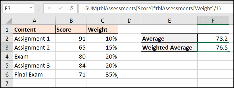
For the final example, we will use the SUM function to help calculate a weighted average.

The following formula is entered into cell F3 to calculate the weighted average of the different assessments and their contribution to someone’s overall score.

=SUM(tblAssessments[Score]*tblAssessments[Weight]/1)

In this formula, we have divided the product of the scores and weights by 1 as the weights total 100%.

It is great that there are different approaches to achieving tasks in Excel. It is one of the things that makes it so much fun.

We are always learning something new and finding fresher ways to do things.