6 Secret Excel Buttons that Many People Do Not Know

In this blog post, we explore the secret Excel buttons that are hidden in plain sight (yes on the Home tab), yet many people do not know them.

There are 6 buttons I would like to mention. They have been ordered both by how useful they are, and almost my view on how aware people are of them.

This list does not even include Conditional Formatting, Clear Cells or the Copy as Picture tool which could all have easily made the cut.

Watch the Video – 6 Secret Excel Buttons

6. Fast Formatting with Cell Styles

The Cell Styles gallery on the Home tab does not necessarily look that useful at first. But it can do some cool stuff.

A cell style is a collection of formatting that can be applied in one click.
You can create your own cell styles by clicking the More button to expand the gallery, and selecting New Cell Style.

In the Style dialog you can assign a name, and then choose the collection of formatting options you want the style to apply.

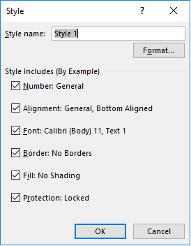
There are lots of good reasons to use cell styles, but I would like to point out two reasons that I favour.

One good use for it is to apply different currency/accounting formats.
It is obviously very popular to have monetary values stored on a spreadsheet, and for some people different currency symbols.

Rather than trawl through the symbol list every time to find the one that you need in that moment. Set it up in a cell style so next time it is just 1 or 2 clicks of a button away.

Another useful reasons is to easily lock or unlock cells when preparing for protecting a worksheet.

It is very popular to lock cells that contain formulas. So set up a cell style with the number formatting, border etc but also the locked setting. Then quickly apply it to cells when needed (check out number 2 for a fast way to select formula cells).

5. Secret Paste Special Options – Repeat Column Widths

Paste Special is an amazing tool in Excel. It is capable of great things and is not necessarily a secret button. However many people are not familiar with all of its potential.

As an example of a secret tip I would like to pick its ability to copy column widths (it is capable of lots more).

This is something that I find very few people know. And it is really useful when it is needed.

Simply copy a cell that has the column width you want to repeat. Then select the column you want to apply that width to. Click Home > Paste list arrow and then Paste Special.

Here you can see all the options at your disposal. Select Column Widths and click Ok.

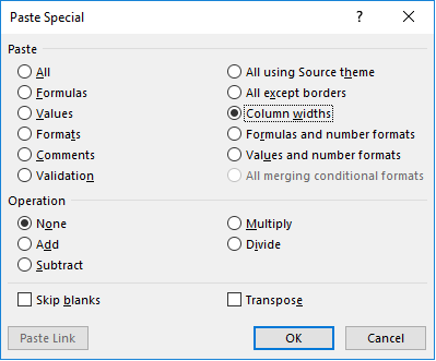
If you want to see more of what it can do, check out my blog post on amazing Paste Special tricks (there is one in this post that very few people know).

4. The Simple, but Dazzling Format Painter

Everyday I find people who are still not aware of the miraculous powers of Format Painter. It is so simple, yet so useful.

How a button that is sandwiched between the Copy, Bold and Font buttons goes unnoticed I do not know. But it does.

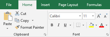
The job of Format Painter is to copy formatting from one place to another. Just the formatting, but all of the formatting. This includes number format, borders, and even Conditional Formatting.

Simply select a cell which contains the formatting that you want, click Format Painter, and then select the cells you want to apply it to.

Tip: Double click the Format Painter button to apply it to multiple cell ranges.

Pro Tip: The Format Painter button even copies formatting between charts (it is not just for cells)

3. Center Across Selection – Do Not Merge Cells

This is probably the least known button in this list. The button is not directly on the Home tab, but its popular alternative is.

And this alternative is the Merge & Center button. Although not a wrong thing to do, this button breaks up the structure of a spreadsheet. This can cause problems and make some tasks awkward.

So do not Merge & Center cells. Use Center Across Selection instead.

The image below is of a header that has been centred (but not merged) across a range of cells.

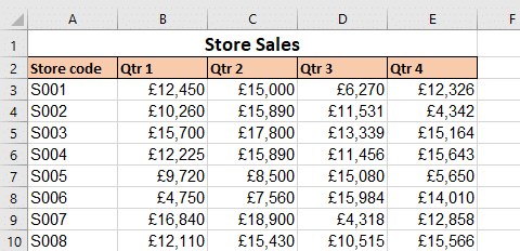
Select the range of cells you want to centre content across. Open the Format Cells menu by pressing Ctrl + 1 or via the right click menu. Select the Alignment tab, and then the list arrow for Horizontal.

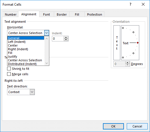
This option is hidden far more than it should be. This frustrates me and I long for the day it sits proudly on the Home tab instead of merging cells.

2. Go To Special Options

This tip ties in very nicely with number 6. Go To Special is a tool that selects all the cells on a sheet that meet certain conditions.

These cells are not always easily visible to us such as cells containing formulas, Data Validation rules or blank cells.

Once selected we can do perform an action such as apply a cell style, delete them, lock them etc.

Go To Special makes it faster, easier and more reliable at selecting those cells.

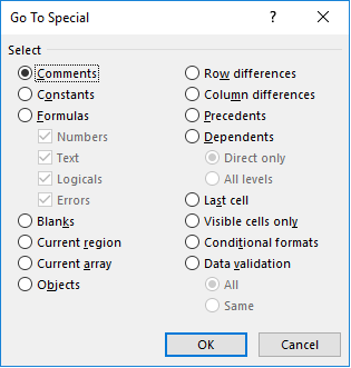
To use it click the Find & Select button on the end of the Home tab. And then either select one of the options in the list, or click Go To Special for the full compliment as shown below.

1. You Must Learn to Format a Range as a Table

Number 1 of the secret Excel buttons is something that I think is very important to get familiar with. And that is formatting a range as a table.

There many benefits to do this, and a lot of them are not all that clear when you are starting out. But there is humungous power and potential with tables in Excel.

It gives your range of cells a meaning to Excel and there opens up a lot of doors to new features such as Slicers and the data model/PowerPivot.

Those features demand a much deeper explanation than what this blog post can offer and learning PowerPivot is encouraged.

To format a range as a table; select a cell in the range and press Ctrl + T, or click the Format as Table button on Home. You can select an in-built style or click New Table Style and create your own.

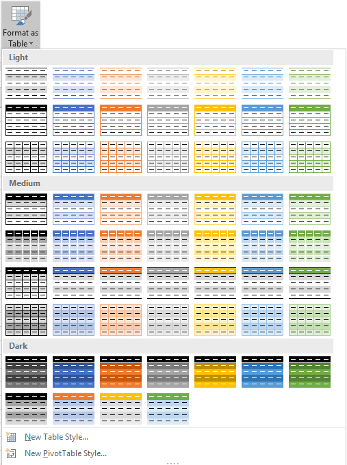
Even without the fancy new ‘Power’ features, formatting a range as a table is beneficial. Advantages include;

• You can assign a name on the Design tab making it easier to reference in PivotTables, Charts and formulas.
• It manages the table formatting for you. If more rows or columns are added, it formats them.
• It keeps the headers visible as you scroll down by moving them into the header area (no more Freeze Panes for this)
• They use structured references for formulas with have more meaning and are more durable than normal cell reference such as D3. An example of a structured reference would be =Customer[Price]*90%.

These benefits are demonstrated in the video at the top of this blog post.

Final Words on the Secret Excel Buttons

So these are my 6 secret Excel buttons that I find many people do not know. And they all sit on the Home tab.

My question is what buttons or features do you find others rarely know of? What secret options that you love and you feel others would benefit from?

Please share them in the comments.