5 Cool COUNTIF Function Examples

The COUNTIF function is one of the most useful functions in Excel. Its job is to provide conditional counting. This is primarily used for analysing data and producing aggregates for reports and dashboards. However, there are many cool COUNTIF function examples in Excel

In this blog post, we will look into 5 more unorthodox but useful scenarios for the COUNTIF function to be used. The 5 COUNTIF function examples we look at are;

1. Prevent duplicates in a range.
2. Uniquely rank items in a list.
3. Count the unique entries in a list.
4. Compare two lists.
5. Identify names that occur 3 times or more.

COUNTIF Function Example to Prevent Duplicates in a Range

Duplicate entries in a list is a common problem to encounter in spreadsheets. By using the COUNTIF function with the Data Validation tool in Excel though we can create a rule to prevent the entry of duplicate values.

In this example we will look at preventing duplicates in range A2:A10.

1. Highlight the range of cells that you want to apply the validation rule to, for example A1:A10.
2. Click the Data tab and then Data Validation.
3. Click the Allow list and select Custom.
4. Enter the formula below into the Formula box provided.

=COUNTIF($A$2:$A2,$A2)=1

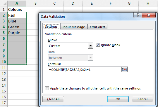
This formula will check if the value being entered is already in the list (equal to 1), and if it is, the Data Validation tool will prevent it from being entered.

Notice the use of the dollar signs to fix the first part of the reference, whilst the row number of the second part of the range is left relative to check all entries in the list.

Uniquely Rank Items in a List

You can rank items in a list in Excel by using the RANK function. For example, you may want to create a league table for your sales team and rank their performance for the month.

However, if two salespeople sell the same amount they will have an equal rank. In the image below two salespeople are ranked in 5^th position and ranking 6 is skipped.

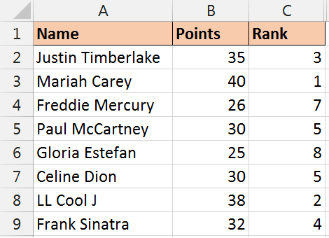
This probably makes sense and is a good thing because they did achieve the same. However if you are planning to create a league table from this data using VLOOKUP, it will not work without a unique ranking for each salesperson.

The formula below creates a unique ranking for each salesperson. It adds 1 onto the ranking if it already exists so that it is not duplicated.

=RANK($C2,$C$2:$C$9,1)+COUNTIF($C$2:$C2,$C2)-1

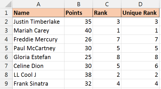
To learn more about creating league tables in Excel, check out our online course for creating sports league tables and competitions.

COUNTIF Function Example to Compare Two Lists

A common requirement in Excel is to compare two lists. There are many different techniques for this, but this article is about COUNTIF.

In the COUNTIF function example below, we want to know what names in the second list do not appear in the first list.

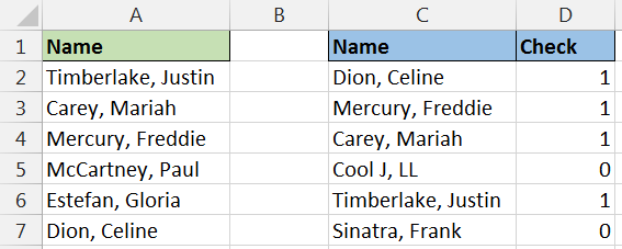
To do this the formula below was entered into cell D2 and then copied to the other rows. It counts how many times the name in the second list appears in the first.

=COUNTIF($A$2:$A$7,C2)

If it returns 0 then the name is missing from the first list. The list can be filtered, used in a PivotTable or have Conditional Formatting applied to work with the results better.

Count the Unique Entries in a List

The COUNTIF function can also be used to create a distinct count (count of the unique entries).

The list below shows the number of visitors to a site. The goal is to find out how many unique visitors there were.

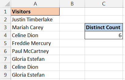
There is no function in Excel for counting unique, or distinct entries. However by combining the COUNTIF function with the brilliant SUMPRODUCT we can get what we want.

The formula below counts the number of unique visitors in the list.

=SUMPRODUCT(1/COUNTIF(A2:A9,A2:A9))

In this formula, the COUNTIF function produces the result below;

{1;1;2;1;1;2;2;2}

This is because Justin Timberlake appears once, Mariah Carey once, Celine Dion twice and so on. So it is counting how many times each delegate attended.

These values are then divided by 1 so that when summed together we are adding 1 for each delegate. The array below is summed.

{1;1;0.5;1;1;0.5;0.5;0.5}

Identify Names that Occur 3 Times or More

Excel provides a few built-in features for handling duplicates in a list including a Conditional Formatting rule. So you will not need the COUNTIF function for this.

However, you may only want to identify the records if they appear 3 times or more in the list, like in the image below.

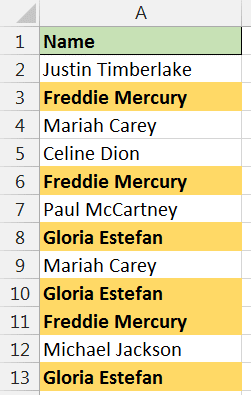
You can write your own rules using formulas in Conditional Formatting. So the last of our COUNTIF function examples is to use it to identify names that occur three or more times.

1. Select the list of names.
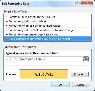
2. Click the Home tab, Conditional Formatting and then New Rule.
3. Select Use a formula to determine which cells to format.
4. Enter the formula below into the box provided.

=COUNTIF($A$2:$A$13,A2)>=3