4 Excel VLOOKUP Examples – Why Use the VLOOKUP Function

When learning the VLOOKUP function, one of the things people can struggle with is seeing why this function is so useful. In this blog post, we look at 4 Excel VLOOKUP examples.

The purpose of VLOOKUP is to look for a value and return some information about that value. Although quite specific in its role, this function can be used in some very clever and interesting ways.

For anyone reading this who may be quite new to VLOOKUP, lets have a quick look at its structure.

=VLOOKUP(lookup_value, table_array, col_index_num, [range_lookup])

• Lookup Value – The value you want to look for.
• Table Array – The table containing the value to look for and value to return.
• Col Index Num – The column number of the Table Array containing the value to return.
• Range Lookup – Optional argument. To specify whether an approximate or exact match on the Lookup Value is needed.

For more information on how to use VLOOKUP, check out the Ultimate VLOOKUP guide.

Watch the Video – Excel VLOOKUP Examples

If you would prefer to watch the video, or simply watch it whilst you refer to the formulas in this tutorial. You can do so below.

1. Easy and Accurate Data Entry

This is one of the more common reasons to use the VLOOKUP function. You can create a lookup table and automate data entry by getting VLOOKUP to fetch it for you.

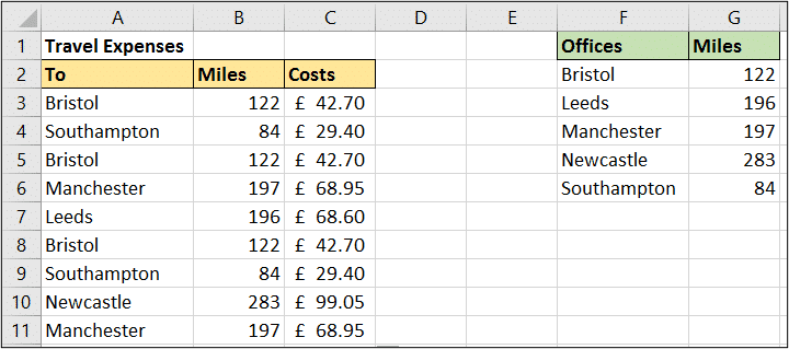
In this simple example we have a travel expense spreadsheet. Someone regularly travels to five different offices. They enter where they went, and need VLOOKUP to return the miles for that office from a table.

The VLOOKUP formula below has been used in cell B3.

=VLOOKUP(A3,$F$2:$G$6,2,FALSE)

2. Complex Logical Formulas

Next in our VLOOKUP examples, is that VLOOKUP can be a great alternative to complex nested IFS and formulas that contain IF and AND to handle their complex logic.

Take this example where the size of the discount increases the higher the quantity you order.

The quantity required and discount qualified for can be seen in columns F and G. Without VLOOKUP this could be a sizeable formula.

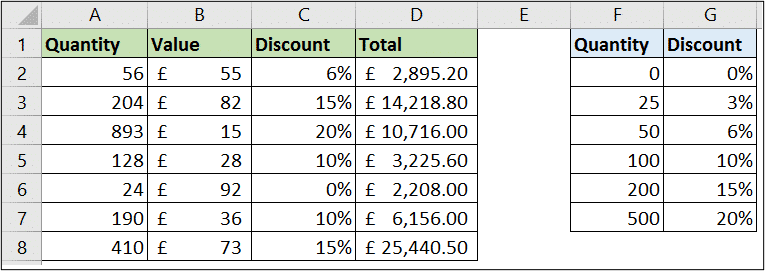
The following VLOOKUP formula is used in cell C2. It uses an approximate lookup, otherwise known as a range lookup, to return the correct discount depending on where the value sits in the ranges of column F.

The TRUE on the end of VLOOKUP is specifying to perform a range lookup.

=VLOOKUP(A2,$F$2:$G$7,2,TRUE)

3. Dynamic Reporting for your Dashboards

A very impressive way to use VLOOKUP is on your reports and dashboards to make your charts and visualisations dynamic.

Lets say you had three tables of sales data like below. As you can see, these are sales of product categories in Canada, Denmark and France.

You have one chart and you would like the user to select which countries data to view from a drop down list.

Well in the image below the drop down list is in cell D2. When the user selects a country from the list, the VLOOKUP’s in column B return the correct data.

Here is the VLOOKUP formula from cell B3;

=VLOOKUP(A3,INDIRECT($D$2),2,FALSE)

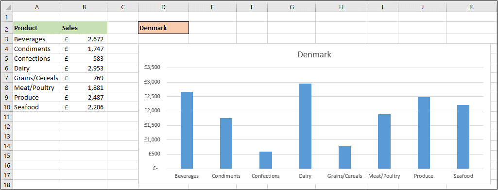
The three tables of data have each been named using the countries name. The INDIRECT function has then been used in VLOOKUP to refer to that table from the users list selection.

4. Compare Two Lists for Missing Values

A very common task for Excel users is to compare lists, and VLOOKUP can help here too. This is the final formula of our VLOOKUP examples.

In this basic vlookup example below, we have two lists of fruit. A VLOOKUP function has been used in a Conditional Formatting rule to identify the fruit that appears in the first list, but not the second.

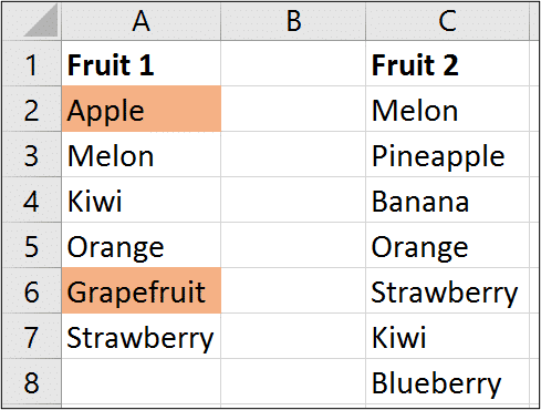
The formula below was used in the Conditional Formatting rule.

=ISNA(VLOOKUP($A2,$C$2:$C$8,1,FALSE))

It uses VLOOKUP to look for the item of fruit from the first list in the second. The ISNA function then reports TRUE if the fruit is not found.

To apply the Conditional Formatting rule;

1. Select the range of cells to format. In this example it was A2:A7.
2. Click Home > Conditional Formatting > New Rule.
3. Select Use a formula to determine which cells to format and then enter the formula in the box provided, and click the Format button to select your formatting options.