The Excel MOD function is used to return the remainder after one number is divided by another. Simple, but there are some very useful examples of the MOD function.
In this blog post, we explore 4 Excel MOD function examples. Hopefully this will help to see how versatile this function can be.
To start we better have a quick introduction to how to use the MOD function. It looks like this;
=MOD(number, divisor)
You need to provide it first with the number you want to divide, and then the number you want to divide it by (divisor).
You can see some basic examples of this below.

Ok, lets get on with some more impressive real-world Excel MOD function examples.
Watch the Video – Excel MOD Function
Here is the video tutorial of the examples explained below.
Extract the Time from a Date and Time Cell
Excel stores dates and times as a number. The time is the fractional part of that number.
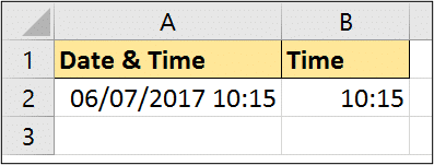
For example, the date and time 06/07/2017 10:15 is stored in Excel as 42922.42708.
Now this does not mean anything to us, but to extract the time part only of .42708 we could use the MOD function and then format the result as time to make sense to us.
The MOD function would be used to divide the number (date and time value) by 1. As this would leave the fractional part as the remainder.
In the example below the following formula was used to extract the time result.
=MOD(A2,1)

This calculation was used in my tutorial to calculate the time elapsed in days, hours and minutes.
Prevent the Entry of Odd Numbers
Another clever example of the MOD function may be to stop the entry of odd numbers in a range.
If a number is an even number, a remainder of 0 would be returned when divided by 2.
It stands to reason then that odd numbers would return a different remainder. We could use this understanding to insert the MOD function into a Data Validation rule.
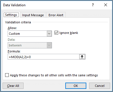
Select the range of cells you want to apply the validation rule to. Click Data > Data Validation.
Select Custom from the Allow list and enter the formula below into the box provided.
=MOD(A2,2)=0
In this formula, cell A2 is the first cell of the range that you selected. This formula ensures that only values that return a remainder of 0 when divided by 2 are allowed.

Total Balls Bowled from Cricket Overs
In my online course on how to create automated sports league tables and tournaments in Excel, I have a section on calculating cricket statistics and league tables.
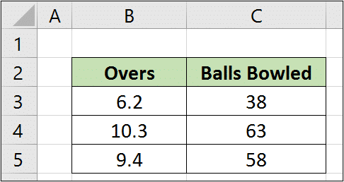
This example comes from that course. We have cells containing the number of overs bowled, but we want to see how many balls is this.
For those who don’t follow cricket. There are 6 balls per over bowled. So if a bowler has made 6.2 overs. They have done 6 overs of 6 balls each and then 2 more balls.
In the spreadsheet below the number of overs is in column B and then the following formula was used in C.
=INT(B3)*6+MOD(B3,1)*10

This formula used the INT function to extract the integer part of column B and multiplies it by 6 to calculate the total balls bowled.
Then the MOD function is used to extract the fractional part (.2 in B3) by dividing it by 1. This is then multiplied by 10 to convert 0.2 to 2. The two parts of the formula are then added together.
Excel MOD Function to Sum the Value in Every nth Row
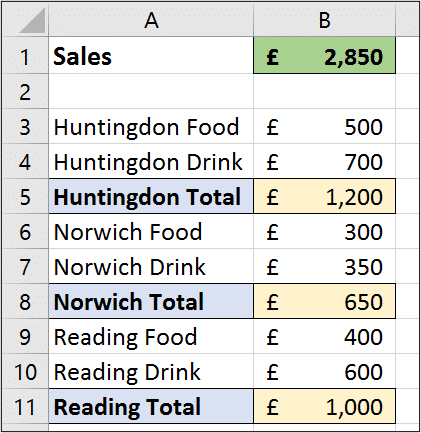
For the final example, we will use the MOD function to help us sum every third cell in a range. This formula can be adapted to sum every other cell, or every fifth cell, or whatever you may need.
This formula uses the impressive SUMPRODUCT function, a favourite of mine.
The formula below uses the ROW function to return the row number of the cell reference starting with B3. A 2 is then subtracted from this because the range starts from row 3. So row 3 is actually row 1 of the range.
The MOD function is then used to divide this number by 3. If the number is divisible by 3 then it must be a multiple of 3.
The number that meet this test in range B3:B11 are then summed.
=SUMPRODUCT((MOD(ROW($B$3:$B$11)-2,3)=0)*($B$3:$B$11))


Leave a Reply