CONCATENATE Function in Excel

The most commonly used text function in Excel is CONCATENATE. This brilliant function joins text together into one cell.

This is typically a combination of written text, and text that is contained in cells on the spreadsheet.

The CONCATENATE function in Excel only requires the different text strings or cell references you want to combine.

=CONCATENATE(text1, [text2], [text3], ...)

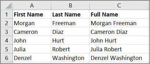
The example below is a typical example of CONCATENATE. In this example, it is being used to join the first name and last name and insert a space in between. The formula below is written in cell C2.

=CONCATENATE(A2,” “,B2)

CONCATENATE Function in Excel with Line Breaks

If you are joining large amounts of text then you may need to wrap it on multiple lines. This is a common technique with text in Excel because excessively wide column can make tables awkward.

To do this with the CONCATENATE function, you must first apply text wrapping to the cells. This alone though will not wrap the text of a formula.

To wrap the text of the CONCATENATE function we need to insert line breaks. And because this is a formula that will require a function.

The function for the job is CHAR. This function will return a character specified by a code from the computer. We need a line break so need to know the code for that. You can find these codes by searching online. For a line break we need code 10.

This CHAR function can be nested within CONCATENATE like below.

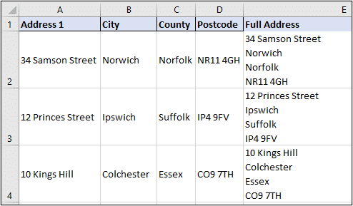
=CONCATENATE(A2,CHAR(10),B2,CHAR(10),C2,CHAR(10),D2)

The result of the above formula is shown below.

You can also Join Text with the Ampersand

The Ampersand (&) can also be used to join text as a simple alternative to the CONCATENATE function. The example below joins the first name and last name again with a space in between.

=A2&” “&B2

Use the TEXT Function to Apply Number Formatting

The TEXT function can be used with CONCATENATE to brilliant effect.

The TEXT function will convert a number to text, but display it in a number format. Without the TEXT function we would not be able to join numbers into a text string in a legible format.

In the example below the TEXT function has been used to include the sum total of values in CONCATENATE, and display them in a currency format.

=CONCATENATE("Total sales for 2016 - ",TEXT(SUM(B4:B8),"£#,###.00"))

CONCATENATE Function for Creative Chart Labelling

Adding descriptive labels to your Excel charts is useful. Adding creative and dynamic labels is awesome.

You can link your chart labels such as the chart title, data labels and axis titles to the cells of a worksheet. The great thing about this is that when the cell content changes, so does the chart label.

Now with CONCATENATE, we can build great content for labels. Take for example, the sales total using the TEXT function we created previously. This would be a great label.

To link a chart label to the cell; simply click on the label, then click the Formula Bar and type = followed by clicking on the cell.

The reference created by Excel will be absolute and include the sheet name. It will look something like =’This Year Sales’!$C$10.

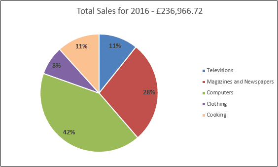
You will then have an awesome chart title like below which updates as the formulas on the sheet change.

More Useful Excel Formula Tutorials

• Extract the Domain from a List of URLs
• 5 Alternative Reasons for using the COUNTIF Function
• Prevent Formulas from Showing in the Formula Bar
• Advanced Techniques for Summing Values