The SUBSTITUTE function in Excel is an awesome text function. It helps us manipulate and work with text strings in Excel.
As its name implies, the purpose of the SUBSTITUTE function is to replace text, or characters in a cell, with different text.
There are some very clever ways that we can put SUBSTITUTE to work.
This blog post explores 3 reasons why we should all love the SUBSTITUTE function in Excel.
If you prefer a video, you can find that below. Otherwise keep reading to see the formula examples.
SUBSTITUTE Function in Excel Examples
Let’s explore the three great examples of the SUBSTITUTE function in Excel.
1. Count the Number of Words in a Cell
There is no function in Excel to count the number of words in a cell. But hey, the SUBSTITUTE function in Excel can help us here.
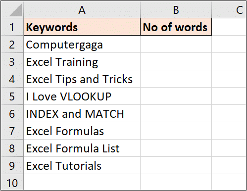
Below are a list of keywords that people may use to find my website. And I want to evaluate how many words are in each keyword string.

Now to do this, we are going to calculate how many spaces there are, and add one on top of that. The logic being that there will always be one more word than there are spaces.
The formula below achieves this.
=LEN(TRIM(A2))-LEN(SUBSTITUTE(TRIM(A2)," ",""))+1
The TRIM function is used to remove all extra spaces from a cell leaving only the one space between each word.
The LEN function is used to count the number of characters in a cell.
The SUBSTITUTE functions role is to replace all occurrences of spaces with nothing.
The resulting formula subtracts a version of the string without spaces from one with spaces. This leaves us with how many spaces there are. We then plus 1 to that result.
2. Change the Decimal Separator with the SUBSTITUTE Function
A question that has come up many times in my training over the years, has been how to handle the different decimal separators used by Europe and the UK (where I reside).
People who work with data from a variety of countries can have complications with Excel’s understanding of the two different number structures.
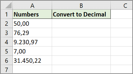
Below are a list of values formatted with the comma decimal separator used in Europe. And our goal is to convert it to a full stop decimal separator used by the UK.
Because of my computers regional settings, Excel does not currently understand what these values are (they are actually stored as text). And obviously I cannot do much with them until Excel understands them correctly.

Great news!
Our friend, the SUBSTITUTE function in Excel can handle this for us.
Below is the required formula.
=VALUE(SUBSTITUTE(SUBSTITUTE(A2,".",""),",","."))
There are 2 SUBSTITUTE functions in this formula. The deepest nested one removes the full stops from the values.
These are being used as thousand separators. But we can do that with formatting so lets completely remove them.
Then the next SUBSTITUTE replaces the comma with a full stop. This is the decimal separator conversion.
The VALUE function then converts it to a number. Because SUBSTITUTE is a text function, the result is always returned as text. So when dealing with numeric values like this, the VALUE function is important.
The Text to Columns tool in Excel provides an even easier way to convert the decimal separators. It is not automated like the formula though.
3. Return the Text after the Last Delimiter
Now for the biggest formula example.
We want to use the SUBSTITUTE function to return the characters after the final instance of a delimiter character.
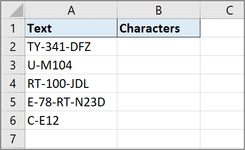
For example, in the list below. We want to return the text after the final hyphen character.

I have also used this technique to extract the postcode from UK addresses successfully.
Now, the first thing we need to do is calculate how many hyphens there are in the cell. Otherwise we cannot determine the final instance of one.
Good news! We have already done that technique in this blog post in example number 1.
Here it is again, but this time counting the occurrences of hyphens (and not spaces).
=LEN(A2)-LEN(SUBSTITUTE(A2,"-",""))
Now that we know how many occurrences of the delimiter character there are. The next step is to put a flag in that final instance to make it unique. The SUBSTITUTE function is up for this job.
In the formula below, an asterisk was used to uniquely flag the position of the final hyphen.
=SUBSTITUTE(A2,"-","*",LEN(A2)-LEN(SUBSTITUTE(A2,"-","")))
We can now use this to extract the characters that occur after this instance of the delimiter.
The RIGHT function will be used for this.
This can be seen in the formula below. The number of characters argument of the RIGHT function has been answered by subtracting the position of the asterisk from the total number of characters.
=RIGHT(A2,LEN(A2)-FIND("*",SUBSTITUTE(A2,"-","*",LEN(A2)-LEN(SUBSTITUTE(A2,"-","")))))
Conclusion
I hope these three examples have established some love for the SUBSTITUTE function (if it did not already exist).
It is a very flexible text function, and especially with the instance number argument is a great utility tool for text manipulation.


Great examples! The SUBSTITUTE function seems really versatile. I especially found the third example useful for replacing specific characters in large datasets. Thanks for the clear explanations!
You’re very welcome. Thank you.
Great examples! The SUBSTITUTE function is so versatile, and I love how you broke it down with clear explanations. I can’t wait to try these out in my own spreadsheets! Thanks for sharing!
Thank you.