3 Excel PivotTable Tips – Common Questions

In this blog post, we will look at 3 PivotTable frequently asked questions. These helpful Excel PivotTable tips are very useful to know.

The three tips are;

1. Changing the PivotTable report layout
2. Editing default PivotTable settings
3. Applying Conditional Formatting to PivotTables

Changing the PivotTable Report Layout

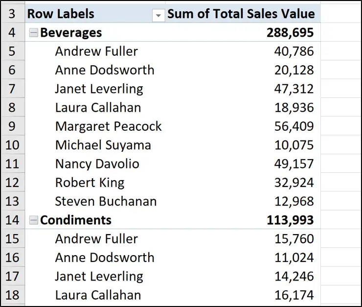
The default layout of a PivotTable is the compact form.

With this layout, the labels sit underneath each other in the same column. The image below shows the sales rep names under the category names in column A.

Some users would like the labels in separate columns. So in this example, categories in column A and the sales reps in column B.

To do this;

1. Click within the PivotTable.
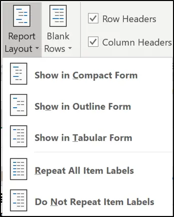
2. Click the Design > Report Layout.
3. Choose the layout you want. In this example, we will choose Tabular Layout.

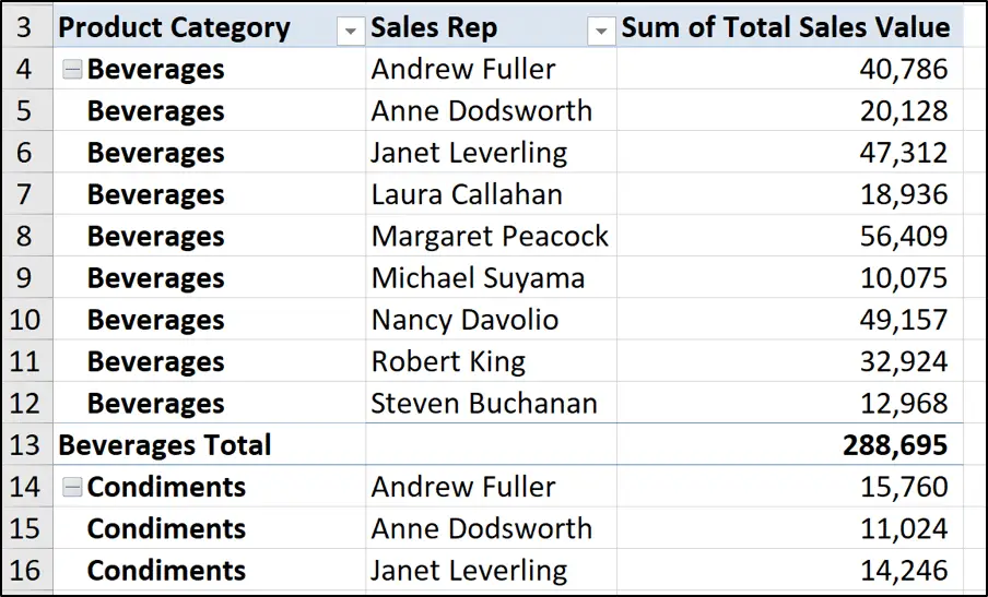
This now positions the different labels from the rows area in separate columns.

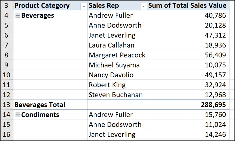
When using this layout, it is common to want to repeat the labels down the column. In this example, the product category is mentioned once and then has several blank rows below.

Click the Report Layout button again and select Repeat All Item Labels.

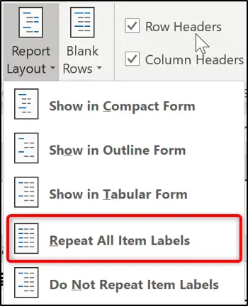
The product category is repeated down column A giving us a complete table.

Default PivotTable Settings

You can edit the default PivotTable settings such as report layout so that you do not need to change them each time you create one.

1. Click File > Options.
2. Click the Data category and then the Edit default Layout button.

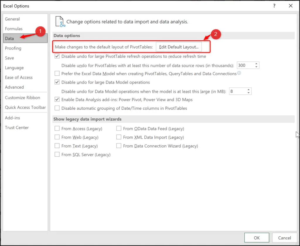
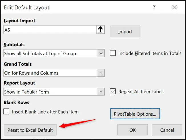
The Edit Default Layout window opens with some useful settings to change.

One of the options here is to change the report layout. This can be changed to Show in Tabular Form. There is also a checkbox to Repeat All Item Labels.

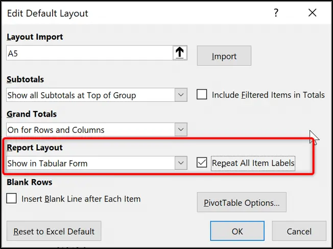
There are other useful options such as if and where you want subtotals and grand totals to be shown as default.

There is also a PivotTable Options button.

Clicking this button takes you to the PivotTable Options window. So it is not just layout settings that can be changed, but also PivotTable options.

Probably the most common option to switch on by default is the Refresh data when opening the file on the Data tab.

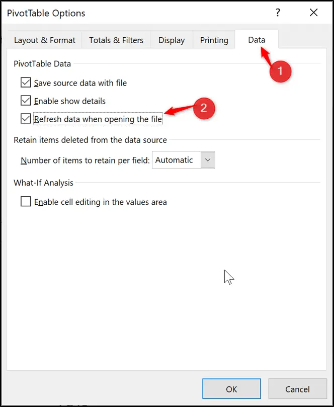
Note: Another common option to change is to stop PivotTable columns resizing on update. Many users find this PivotTable behaviour frustrating.

Click OK to save these changes and the next time you create a PivotTable, these settings are automatically applied.

If in the future you want to restore your PivotTable settings back to what they were, you can click the Reset to Excel Default button in the Edit Default Layout window.

Conditional Formatting with PivotTables

I am often asked if you can apply Conditional Formatting rules to PivotTable data. Well, sure you can.

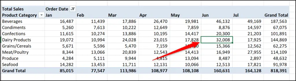
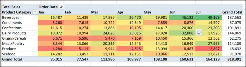
Let’s add a Color Scale rule to the PivotTable below. Start by clicking a single value in the PivotTable.

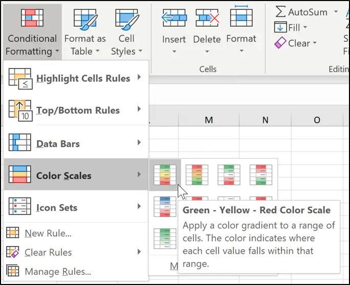
Click Conditional Formatting > Color Scales > and select the Green – Yellow – Red Color Scale.

The Conditional Formatting is applied only to the single selected cell.

But a small icon also appears next to that cell. Click the icon to see options for what values the Conditional Formatting rule is applied to.

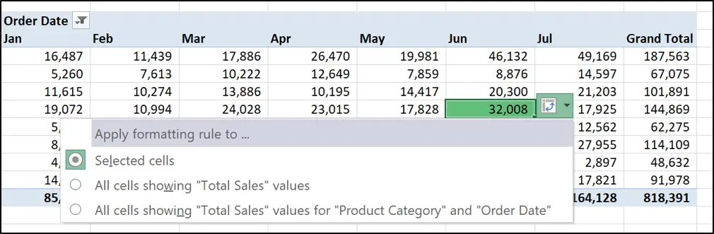
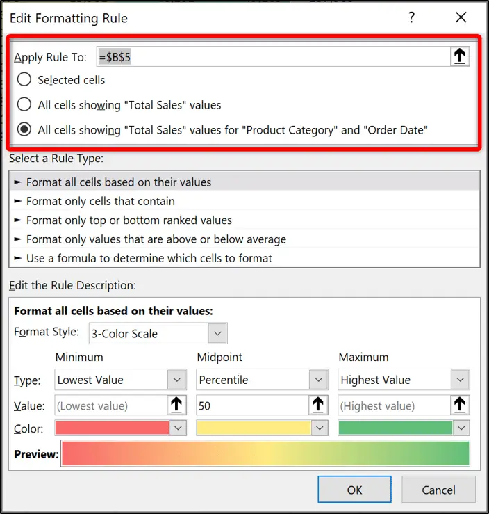
In this example, we want to select All cells showing “Total Sales” values for “Product Category” and “Order Date”.

This will ensure that the grand total values are not taken into account. But also, as more months are added to the PivotTable, the Conditional Formatting will automatically pick these new values up.

You can also access the options for which values the Conditional Formatting rule is applied to when editing the rule.

1. Click in the PivotTable.
2. Click Home > Conditional Formatting > Manage Rules
3. Select the rule and click Edit Rule.

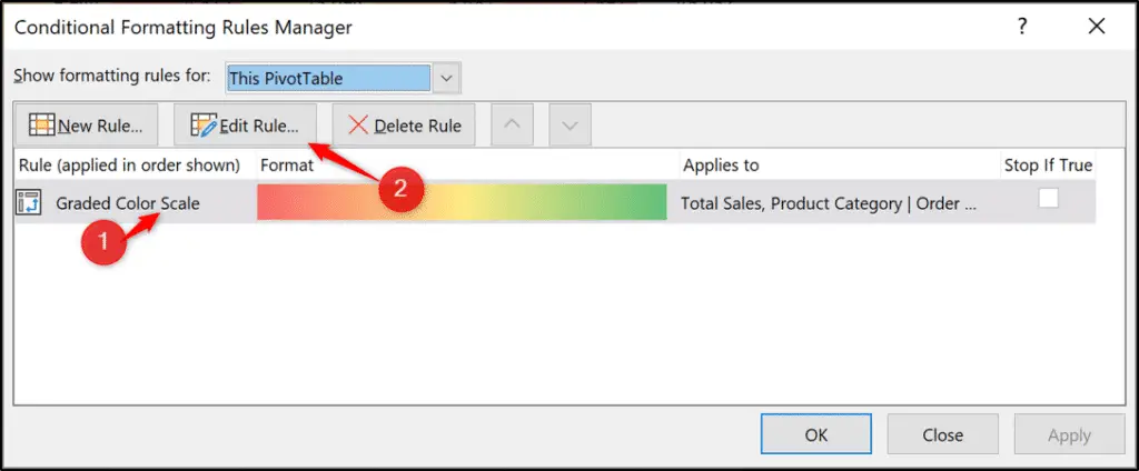
The option to change which values the rule is applied to can be seen at the top of the window.