Create a Picture Lookup in Excel

Many Excel users are familiar with lookup functions such as VLOOKUP, INDEX and MATCH to look up information in a list. But how about performing a picture lookup in Excel to return a picture dependent upon the contents of a cell.

This requires a little extra thought as a standard VLOOKUP is not capable of returning a picture from a list.

In this blog post, we will explore how to create a picture lookup. We will look at how to return the picture of a flag dependent upon the country name that is selected from a list.

Spreadsheet Setup

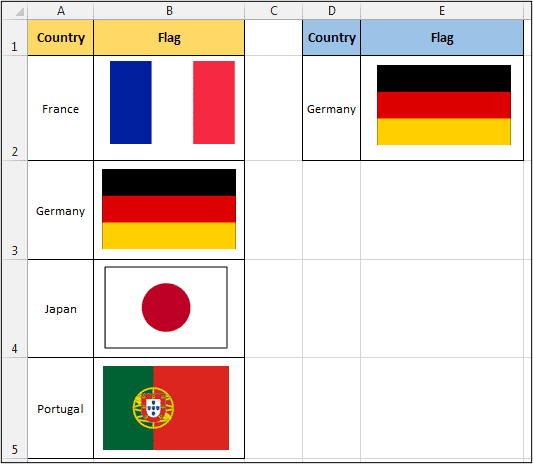
In this example we have a list of countries and their flag. It is very important in this list that the picture (flag), is completely inside the cell. You can see the white space between the frame of the picture, and the borders of the cell containing it.

Cell D2 contains a drop down list with each countries name. When a country is chosen we wish for the corresponding flag to be returned.

Although a drop down list is used in this example, the data used for your lookup can be the result of any formula, or data entry method.

Create a Picture Lookup in Excel

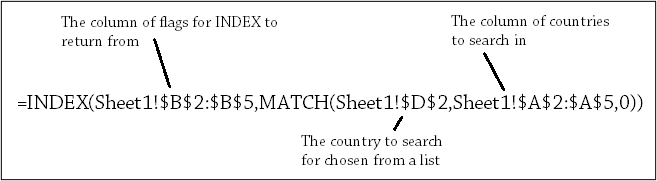
As it is not possible to write a lookup function in a cell to return the picture, we will enter the formula into a defined name. The INDEX and MATCH functions have been used to perform the lookup.

1. Click the Formulas tab on the Ribbon and then the Define Name button.
2. Enter a name for the defined name such as FlagPic
3. Click in the Refers to: field and enter the following formula.

=INDEX(Sheet1!$B$2:$B$5,MATCH(Sheet1!$D$2,Sheet1!$A$2:$A$5,0))

Linking the Picture to the Formula

Now we need to link the picture in cell E2 to the defined name.

1. Select the picture.
2. Enter =FlagPic (or whatever name you used) in the Formula Bar and press Enter.

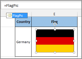
And that is it. When a different country is chosen from the list in cell D2, the appropriate flag is returned.

Watch the Video